Project 4: Cloth Simulation
Ashley Nguyen | CS184-agh

The Blue Umbrella
Overview
In this project, I implement a real-time simulation of cloth using a mass and spring based system. I built the data structures that discretely represent the cloth, define and apply physical constraints on them, and apply numerical integration to simulate the way cloth moves over time. Finally, I implement collisions with other objects as well as self-collisions to prevent cloth clipping.
Part 1: Masses and springs
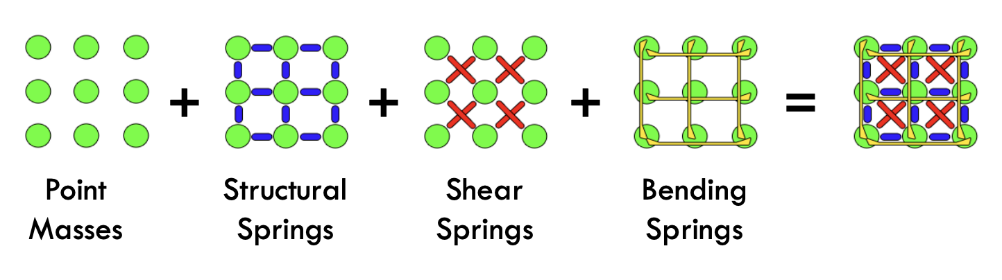
In this part of the project, I build the physical model of the cloth. To do this, we include the grid of masses and springs. Given the dimension and parameters, we build evenly spaced point masses and connect neighboring masses with springs.
To build the grid of masses and springs, I start by producing the evenly spaced point masses. For this I use num_width_points and num_height_points for the number of point masses that will span the width and height. Based on the orientation, we set the coordinates differently. If the orientation is HORIZONTAL then we set the y coordinate to 1 and the position is set on the xz plane. It the orientation is VERTICAL then we set the z coordinate to a random number between [-1/1000, 1/1000] and the position on the xy plane.
Lastly, we create springs between the point masses. We create structural constraints between a point mass and the one on its left and above. We also create shearing constraints between a point mass and the one above diagonally to the left and right. Finally, we create bending constraints between a point mass and the point mass 2 point masses away to its left and above.
Level N-1
Below are rendered photos of a cloth wireframe. Each show the wireframe with different constraints.
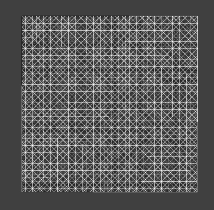
cloth wireframe - with all constraints
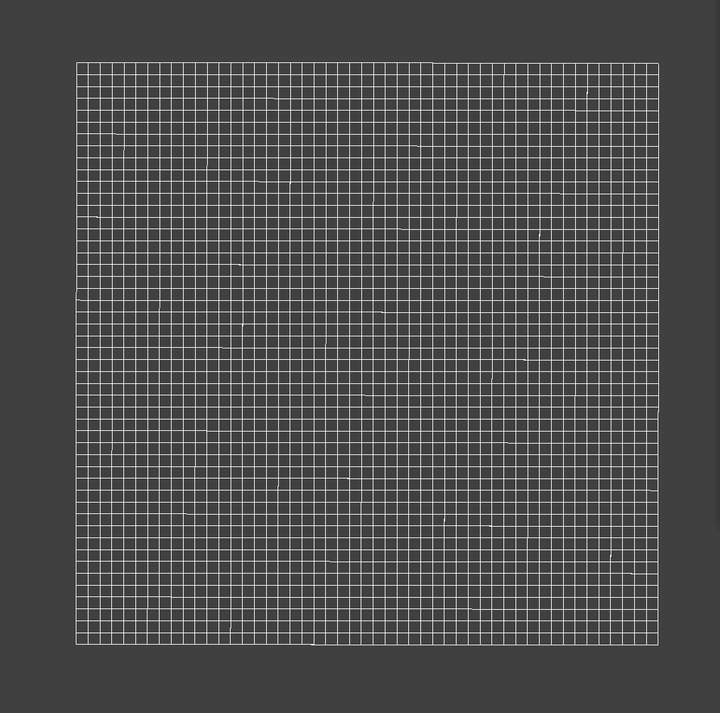
without shearing
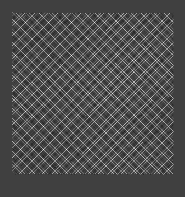
only shearing
Part 2: Simulation via numerical integration
In this part of the project, we integrate the physical equations of motion to apply the forces on the point masses. We calculate how they move from one time step to the other. We first need to calculate the forces on each point mass. We calculate the total of all the external accelerations. Then we apply the spring correction forces using Hooke’s law. Then we adjust the actual positions of each mass using Verlet integration to approximate the position at this next time step. To make sure the positions don’t stretch we make sure the spring length is at most 10% more of the rest_length.
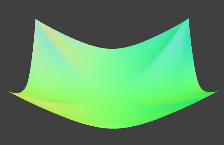
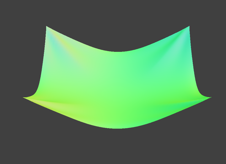
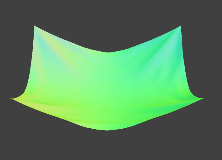
When experimenting with the parameters, we see the final rendered image looks different.
Spring Constant (k_s)
When we change the spring constant parameter, we see the cloth looks tighter and the elasticity changes as we increase or decrease the density. The lower the spring constant the more elastic it becomes. The higher the spring constant the tighter and less elastic the cloth is.
k_s = 500

k_s = 5000
k_s = 50000
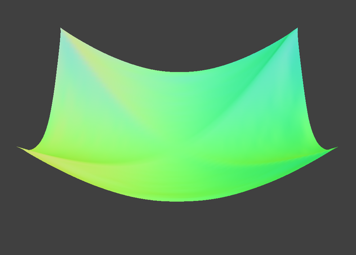
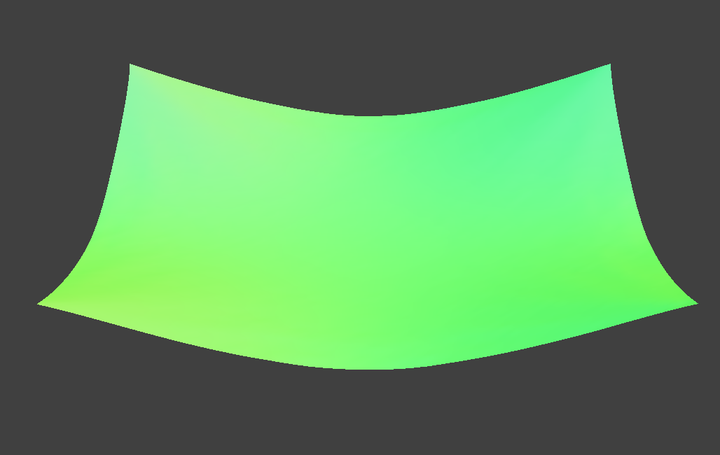
Density
When we change the density parameter, we see a change to the cloth opposite to the spring constant. We we the higher the density the more the middle of the cloth dips in. This indicates that it is less stiff and is more malleable when pinned.
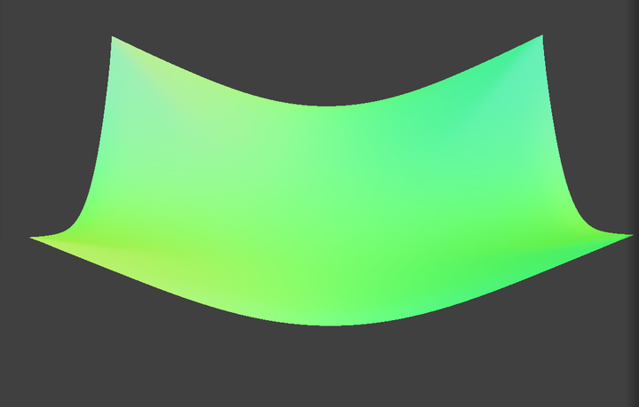
density = 7.5 g/cm^2
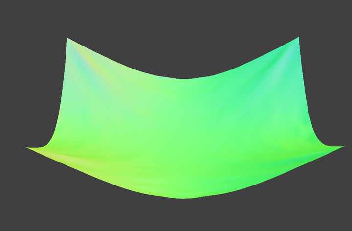
density = 15 g/cm^2
density = 30 g/cm^2
Damping
When we change the damping of a cloth, the final stage is very similar to each other. However, the damping parameter varies through the process of the cloth falling. When damping is low the cloth falls faster. It swings and wrinkles more. When the damping is high the cloth slower and swings less.
damping = 0%

damping = .2%
damping = 1%
Below is the image of the cloth with the preset parameters when the cloth is pinned on all 4 corners
Part 3: Handling collisions with other objects
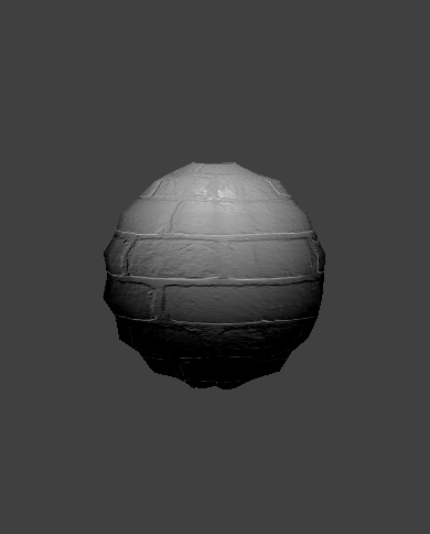
In this part of the project, we calculate collisions of the cloth with various objects. We do this by testing if the point on the cloth lies on or inside the object. If it does then we move the point above the object. We do this by calculating the tangent point along the object based on the vector formed from the last position to the current position. (Or if the object is a sphere then we use the vector from the center of the sphere to the current position.
Below are rendered images of a cloth covering a sphere. In this we include various ks values.
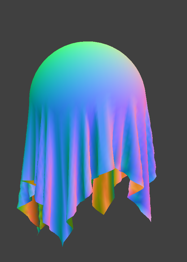
ks = 50
ks = 500
ks = 5000
ks = 50000
ks = 500000
As we increase the spring constant, we notice that the cloth becomes stiffer and there are also less folds. As we decrease the spring constant, we notice the cloth wraps around the sphere and there are more folds.
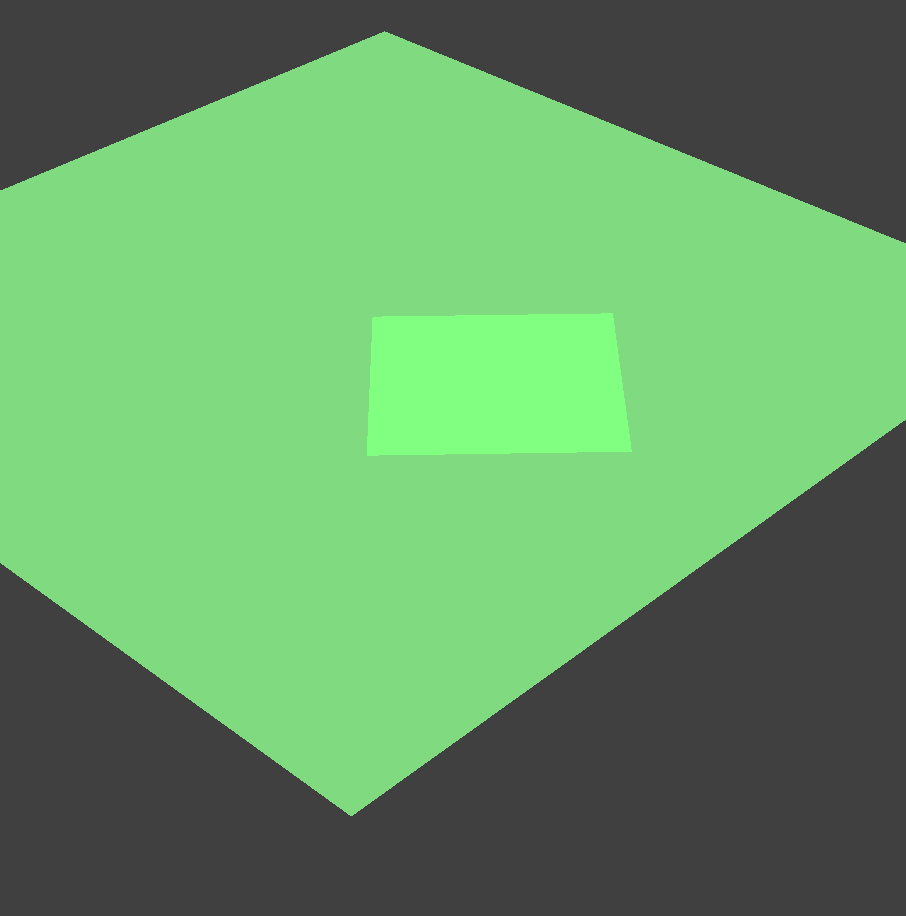
cloth on plane
Part 4: Handling self-collisions
In this part of the project, I handle the case where the cloth self-collides. Before this part, the cloth will fall on itself and clip through and behaves unnaturally. The cloth falls on itself, ignores itself, and then falls on the plane.
To do this, we implement the spatial hashing. At each time step, I build a hash table which maps a float to a PointMass vector. The float represents some point in the 3D map. Using the map, we loop through the PointMasses, find the PointMasses each PointMass shares the 3D volume with and apply repulsive collision force the the pair is close.
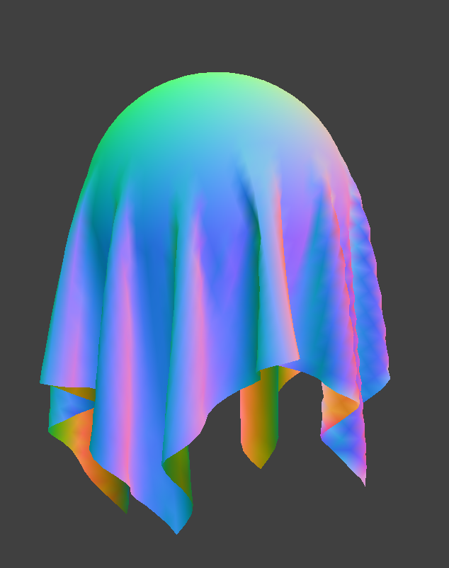
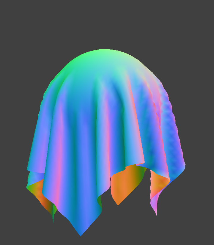
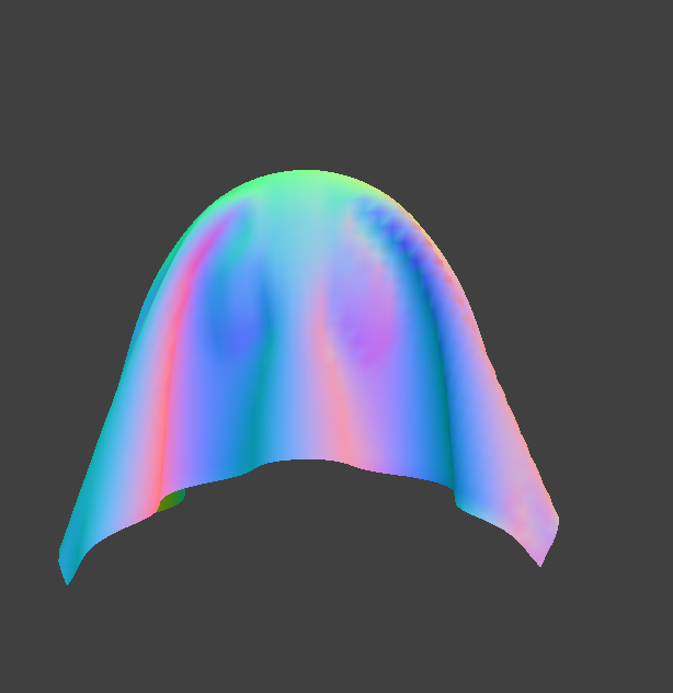
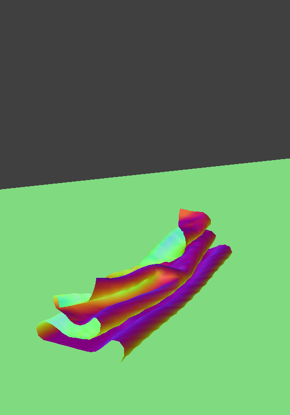
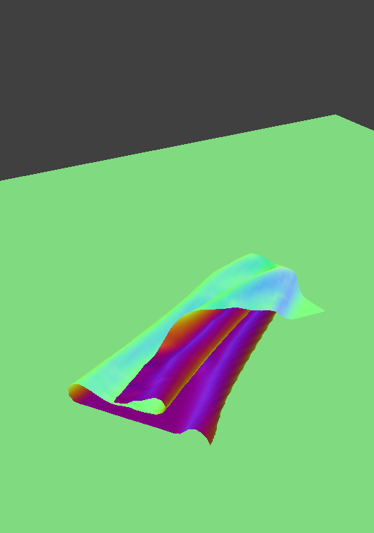
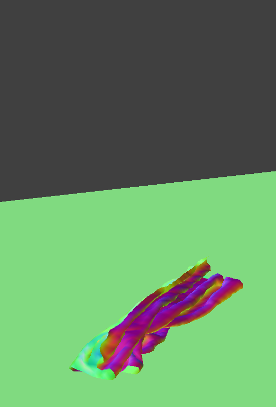
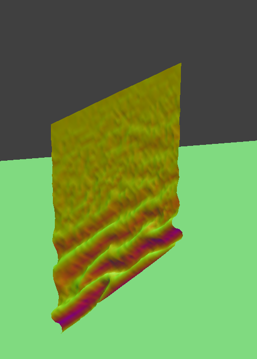
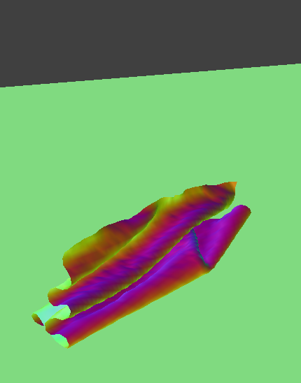
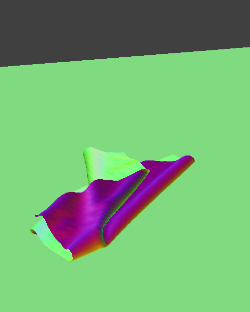
Below are rendered images of the cloth with varying parameters.
Spring Constant
ks = 50,000
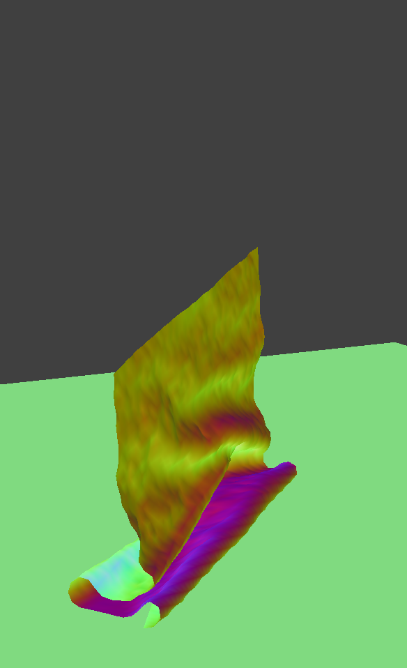
start
mid
final
ks = 5,000
start
mid
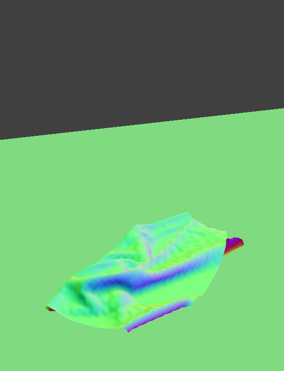
final
ks = 500

start
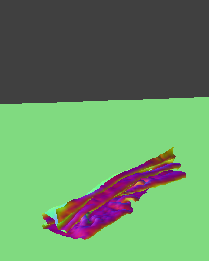
mid
final
As we decrease the spring constant, the cloth falls with more wrinkles and more folds. The cloth looks more crumpled but at the end unfolds itself. As we increase the spring constant, the cloth falls with less but bigger folds. The cloth is more stable and stiffer. The final state looks crispier and has more folds.
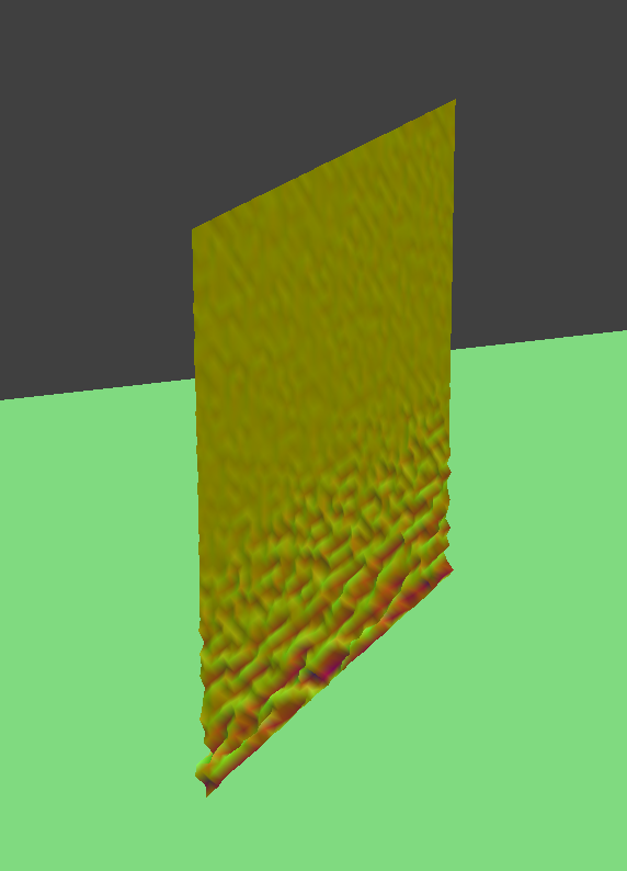
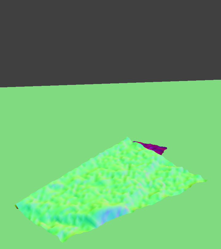
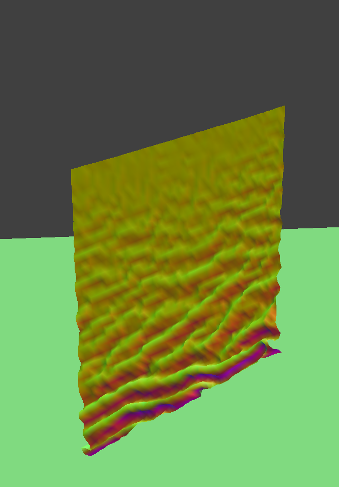
Density
Density = 1.5g/cm^2
start
mid
final
Density = 15 g/cm^2
start

mid
final
As we decrease the density, we get the same effect as increasing the spring constant. The cloth looks more crumpled but at the end unfolds itself. As we increase the density, the cloth falls with less but has bigger folds. This effect is similar to decreasing the spring constant.
Part 5: Shaders
In this part of the project, we create GLSL shader programs to accelerate the time it takes to render a frame with realistic lighting. We implement Diffuse, Blinn-Phong, Texture Mapping, Bump & Displacement Map, and Mirror shaders.
OpenGL allows us to define shaders. These shader programs run in parallel on the GPU which allows you to define different steps of the rasterization pipeline. There are 2 types of basic OpenGL shaders: a vertex shader and a fragment shader.
Vertex shaders generally apply transforms to vertices that effect the geometric properties. This includes the position and normal vectors. This helps with making a bumps and the overall geometric shape of the objects look realistic.
The fragment shader takes in the properties of a fragment calculated by the vertex shader and computes a color using shading models.
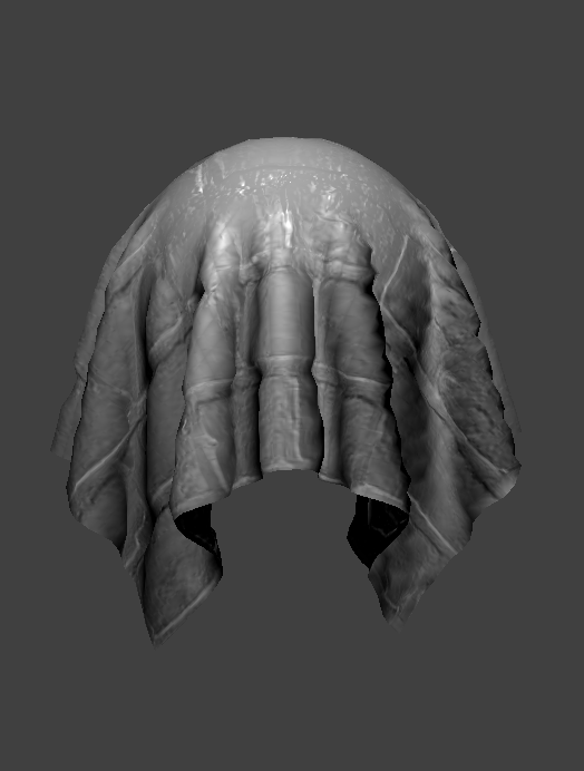
One of the shading models we use is Blinn-Phong. This computes the fragment color using an ambient light component, a diffuse component and a specular reflection component.
Below are rendered images of the cloth on the sphere. In the examples above we isolate each component mentioned in the Blinn-Phong model.

only ambient light component
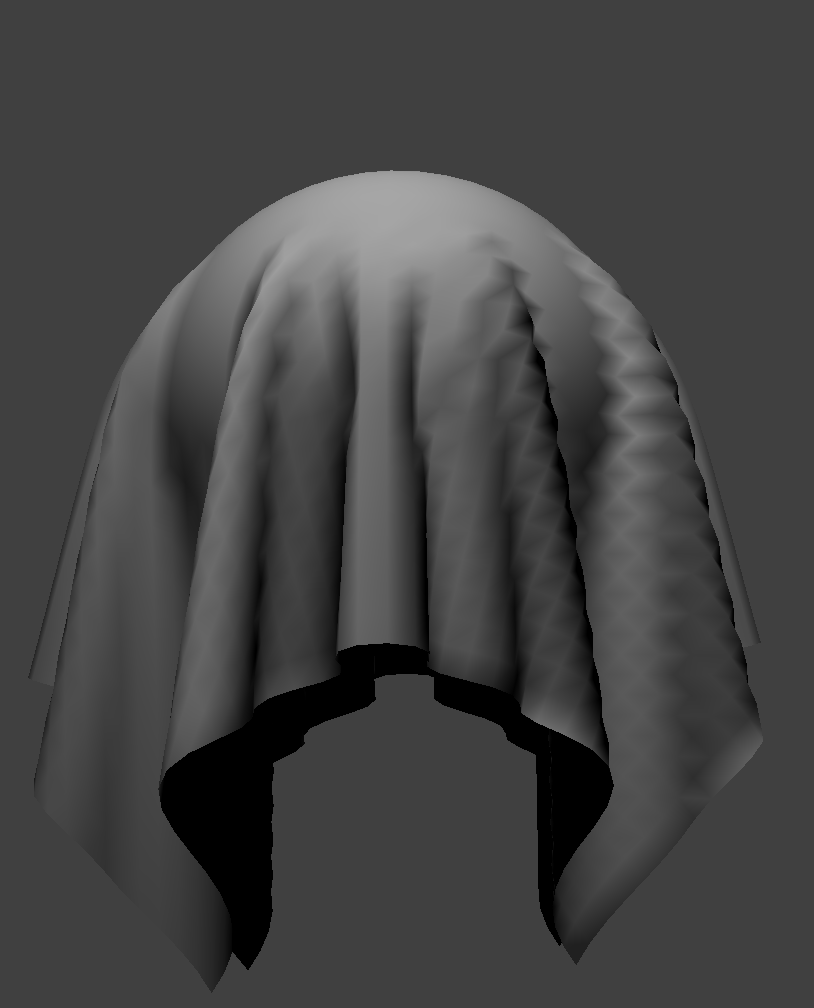
only diffuse component
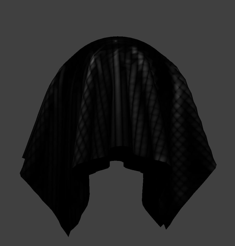
only specular component
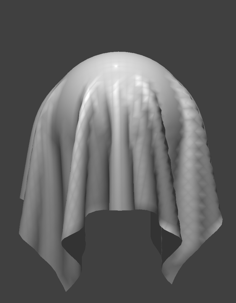
Blinn-Phong model
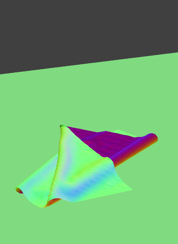
Below is a rendered image of the texture mapping shader.
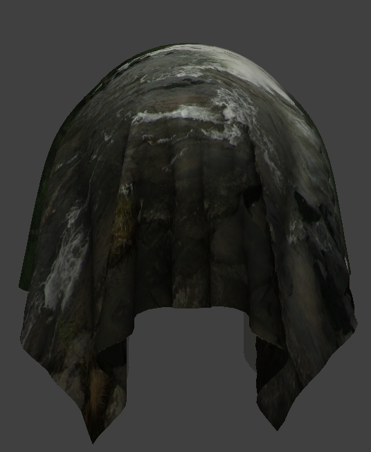
Storforsen
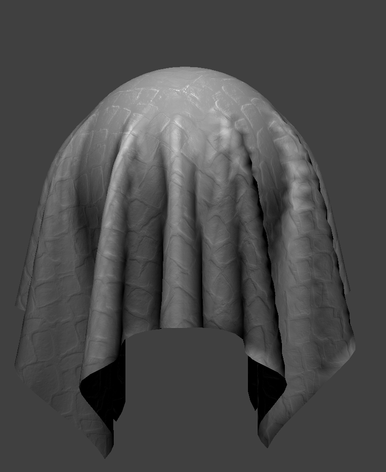
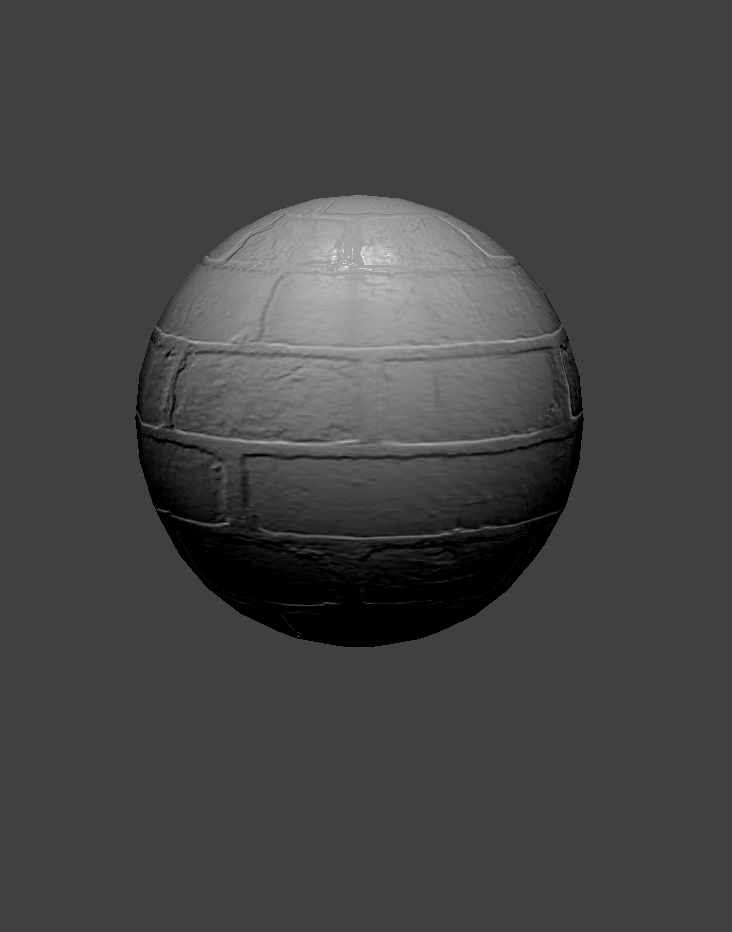
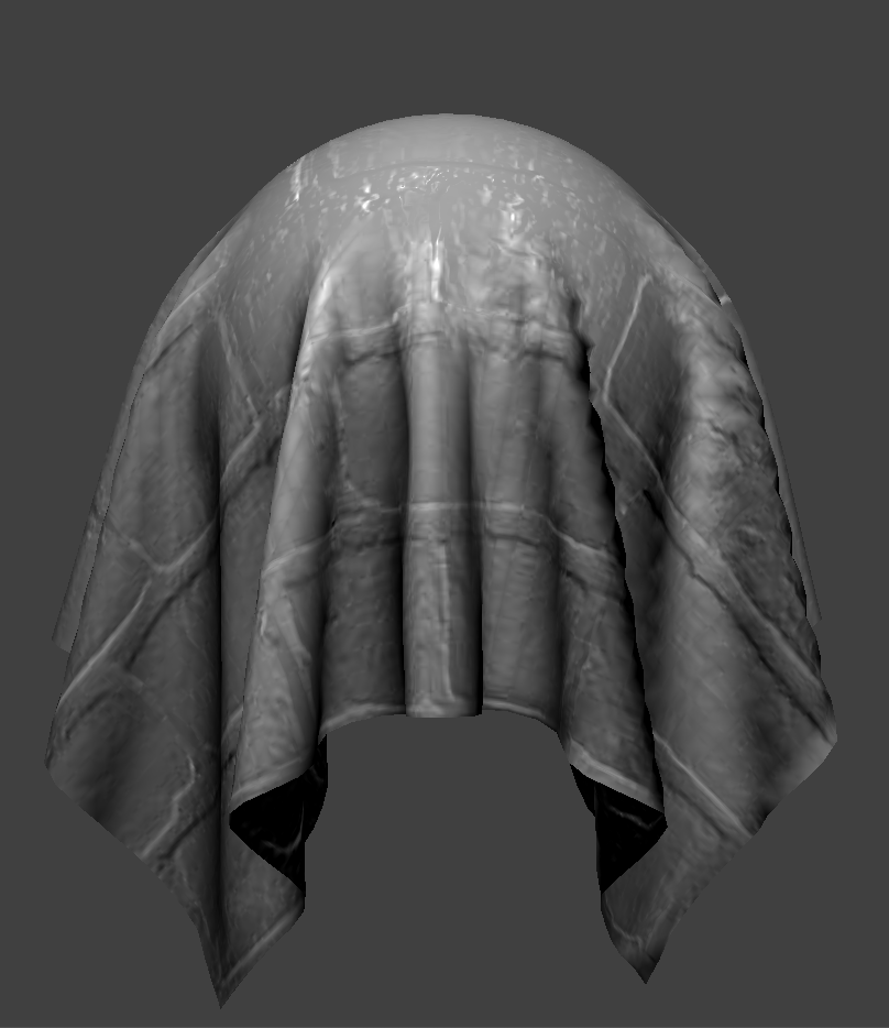
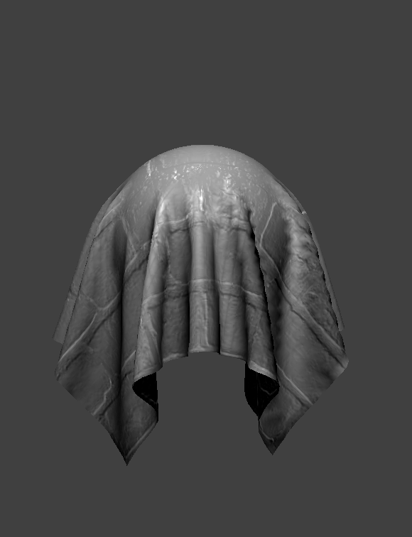
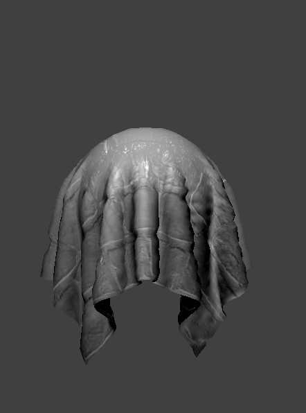
Below is a rendered image of bump mapping on the cloth and on the sphere.

In the next render, I compare the bump mapping on the sphere with the displacement mapping on the sphere. Looking at the 2, side by side, we can see the 2 objects have relatively the same outline. However, you can see with the modifications in displacement, it displaces the geometry and so the positions of the vertices of the fragments have changed as well.
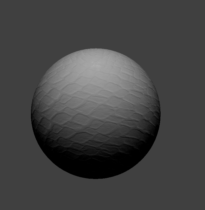
bump
displacement
Next, I compare how different shaders act differently when the mesh’s coarseness is modified. I use the parameters -o 16 -a 16 and then -o 128 -a 128.
coarseness 16
coarseness 16
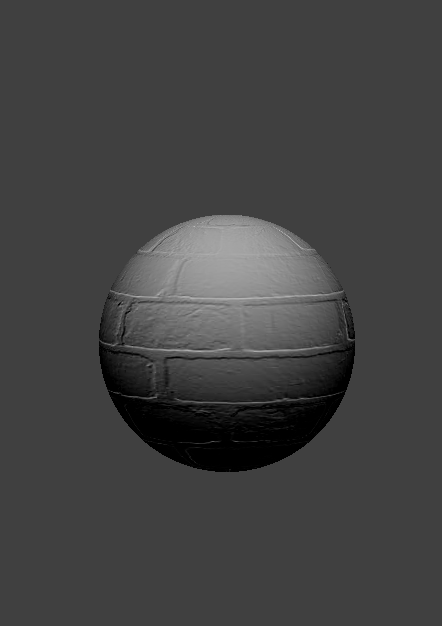
coarseness 128
coarseness 128
There is very little change between the 2 images. The light that shines on the sphere when the coarseness is changed to 128 looks more diffused. In addition, the sphere on the right looks more realistic and sharper.
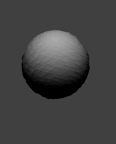
Below are renders of the displacement mapping shader with various coarseness.
coarseness 16
coarseness 16

coarseness 128
coarseness 128
The displacement in the mesh that has a higher coarseness is very obvious. The higher the coarseness the more displacement we get of points. The lower the coarseness the less coarse the mesh is.
Below is a rendered image of the mirror shader on the cloth and on the sphere.
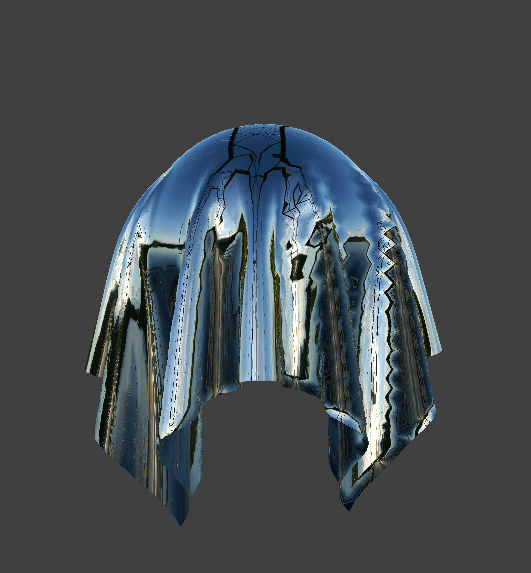
Mirror