Project 1: Rasterizer
Ashley Nguyen | CS184-agh
Overview
In this project, I convert an image vector using linear algebra concepts into a rasterized image. From basic coloring pixels to supersampling, transformations, and texture mapping with antialiasing, I discover how different methods of rasterizing can help change the form or quality of an image.
Section I: Rasterization
Part 1: Rasterizing single-color triangles
So what makes a triangle. By definition, a triangle is a polygon that has 3 sides with 3 angles whose angles all add up to 180°. Each side on a plane can be represented as a line equation (y = mx + a). Some helpful linear algebra concepts in this section are line derivation and line inequalities I first begin the project with a simple algorithm to rasterize a triangle. I bound the triangle by a box that equates to the min and max of the vertices. Then I go pixel to pixel and test if the center of the pixel is within the 3 lines that make up a triangle. To do this I use the intersection of 3 planes and use the point-in- triangle test if the testing point is less than or equal to (<=) or greater than or equal to (>=) than all the lines.
Here is a visual example of the 3 line inequalities. It is very subtle but the inside of the triangle is darker than the rest of this plane.
The reason for checking if the point is all = to any of the lines is if it is a literal edge case. In this method I consider an edge case as a pixel within the triangle. If the center of the pixel meets the point-in-triangle test then i use fill_color() to color the whole pixel. Below is an example of an image generated using this method of rasterization.
Basic rasterization using point-in-triangle test.
Here you can see a problem when zoomed in. These jaggies don’t create a quality image and although it can not be perceived when the pixel size is small but it is very obvious when zoomed in. We will visit a solution in the next section.
Ways I’ve optimized this solution was by creating 2 helper functions flat_bottom() and flat_top(). The structure of these functions are similar to the one I explain above but instead of looping through a box shape I change the length of the row of pixels I check by calculating the slopes of the sides of the triangles that are not flat. Using these 2 functions, I can solve any triangle. First I sort the vertices by y values then split a triangle that does not have a flat edge at the 2nd highest y value. This creates 2 different triangles: one with a flat bottom and one with a flat top. Then I could use the flat_bottom() and flat_top(). This optimizes the number of pixels the functions tests.
Part 2: Antialiasing triangles
In the previous part, I found that by just checking the pixel just once creates jaggies that doesn’t make the image look pleasing. A solution to this problem is testing the pixel multiple times and taking the average of all the pixel samples. This will prevent the jaggies and create a more blur looked to rather than sharp color changes. Concepts important to this part of the project are antialiasing and supersampling.
In order to make the edges look smoother, I use supersampling to average the sub_pixel colors and set the pixel equal to that average. Essentially what I am doing is weighing how much of each pixel is within the triangle. Below, I include a visual representation that would better explain my process.
I divide the pixel into sub_pixels based on the sample_rate and then use the point- in-triangle test on each sub_pixel.
After testing each sub_pixel, I average all the sub_pixel colors and set the pixel color to the average.
The example above shows the process of breaking each pixel into sub_pixels based on the sample_rate which is 4 (2x2 sub_pixels). Then, on each sub_pixel I test the center of the sub_pixel using the 3 line inequalities to see if the sub_pixel is inside the triangle. After doing so, I take the average of all the sub_pixels and set that color value to the main pixel. So instead of getting the jaggies, we see pixels that are not entirely in the triangle with a lighter color.
To better represent how supersampling prevents jaggies from happening I include a picture with various sample_sizes.
sample_rate = 1
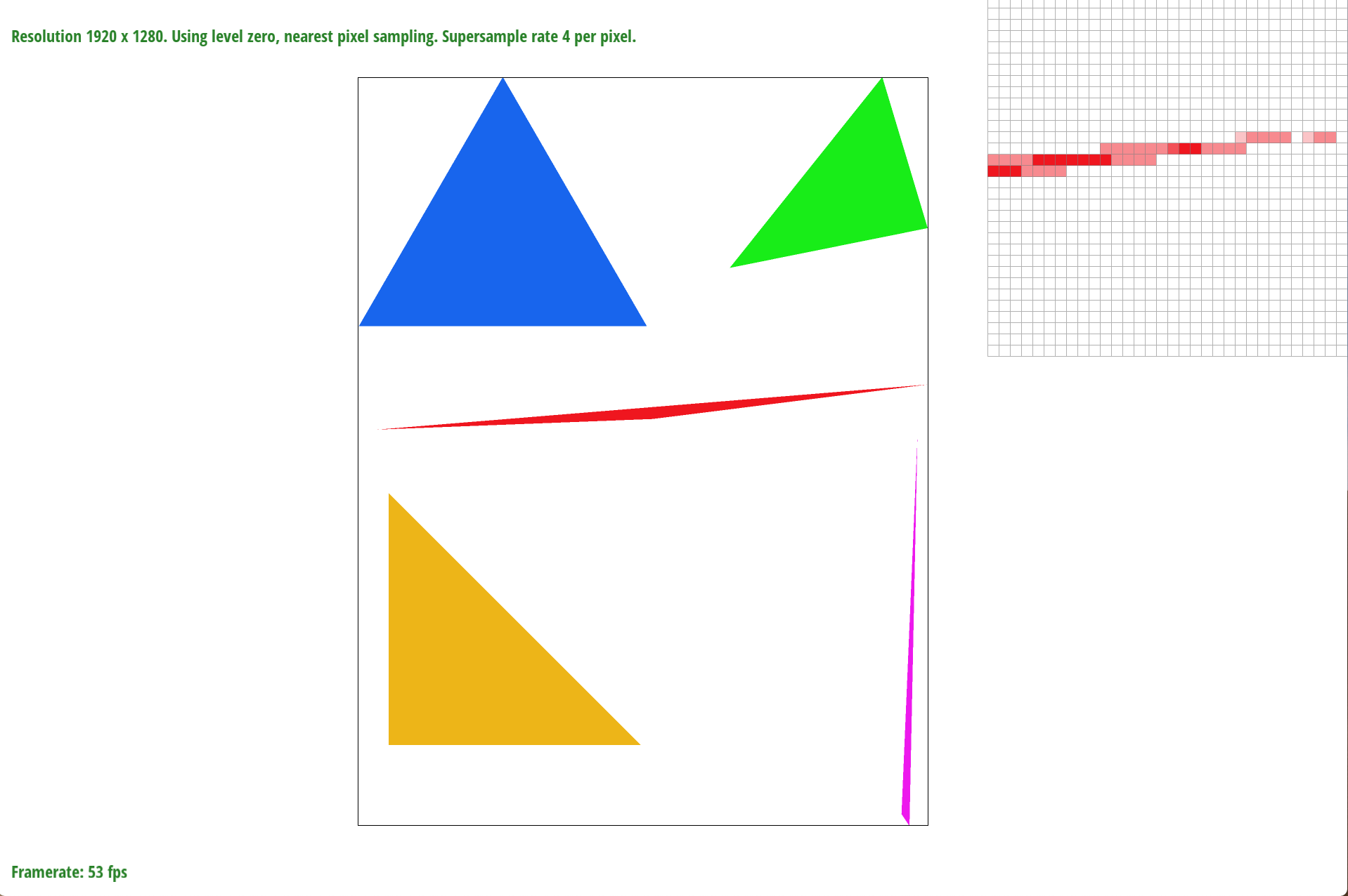
sample_rate = 4
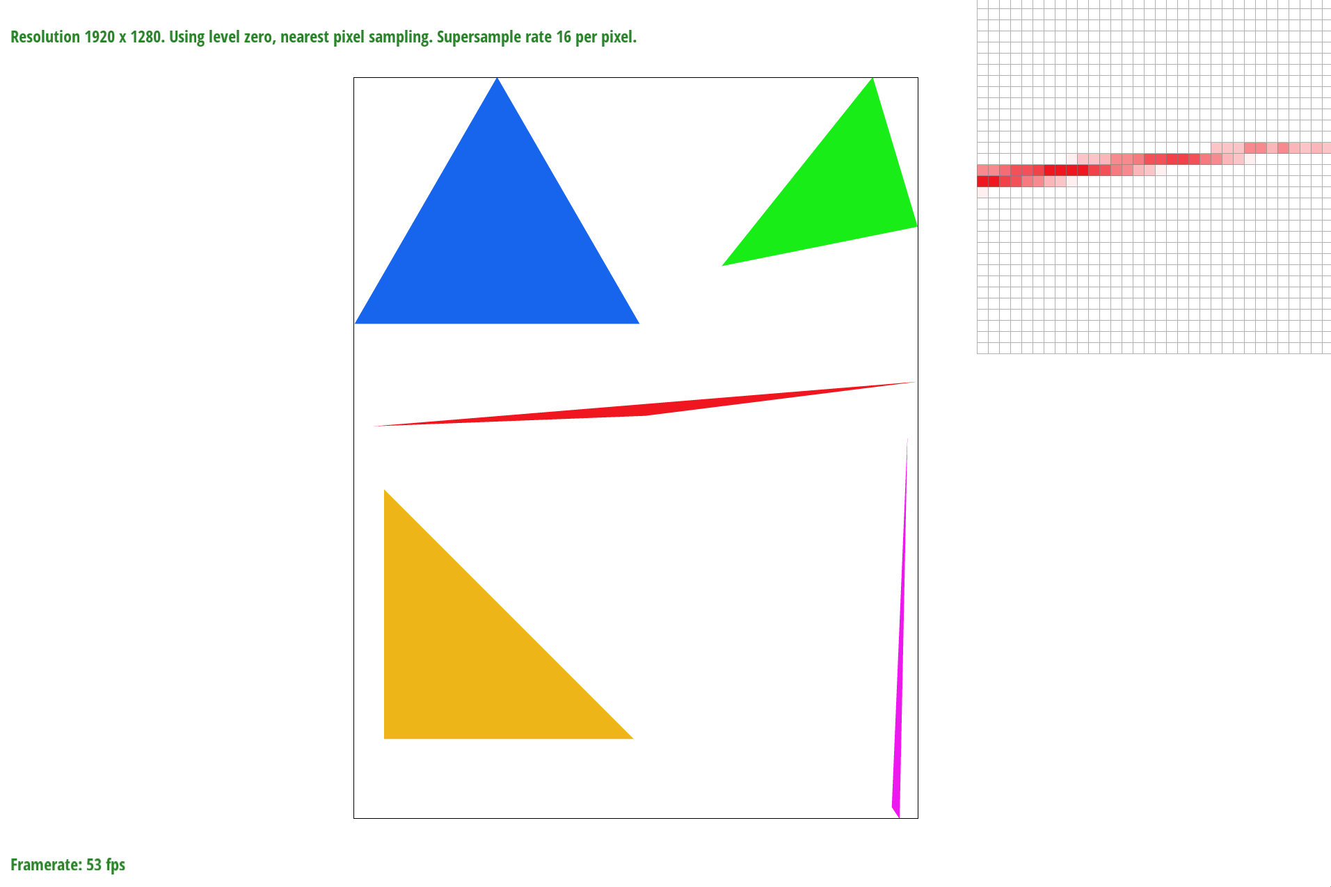
sample_rate = 16
Here you can see how the sample_rate creates a better image the higher the rate is. By antialiasing images, we have smoother edges as oppose to the jaggies.
Modifications for testing the sub_pixels were made in the main rasterization and modifications to coloring the pixels were made by swapping the function I used to color the pixel with a function that returned an average of the sub_pixels.
Part 3: Transforms
Another cool part of manipulating shapes is through transformations which include but are not limited to rotation, scaling, translating, etc. In this part of the project, I concentrate on rotating, scaling, and translating. Important concepts in this part include homogeneous coordinates and composing transforms.
To demonstrate, these transformations in action, below I include a manipulation using these matrices.
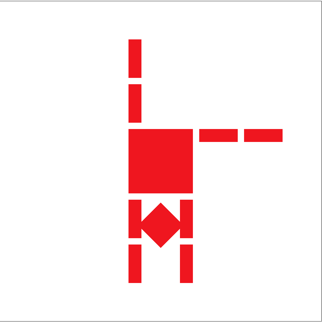
Robot doing a handstand
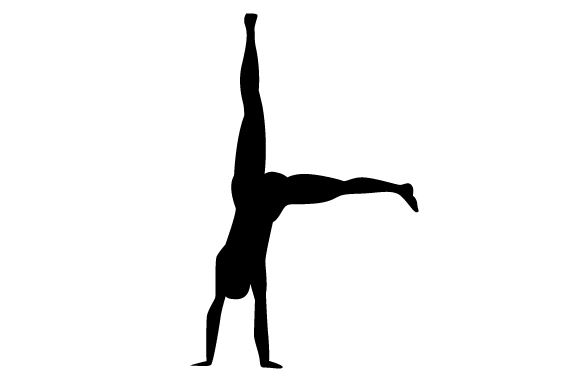
model
Originally, the robot was standing right side up with its arms out. In this example, I translate the head of the original robot down. What are now the legs of the robot, I rotate each part of the leg to point up then translate each part to the correct spot. Using these transform matrices, I can manipulate shapes to create a new images.
It is necessary to include the third coordinate even though we are working in the 2D space because transformations like translation are not linear transformation. So by creating homogeneous coordinates we are able to perform nonlinear translations.
Section II: Sampling
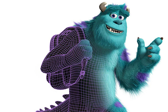
In this section of the project, we are working with image textures. The difficult part of working with textures is finding the texture coordinate mapping from the 3D object to the image. Below is an example of what texture coordinate mapping of an image onto a 3D object looks like.
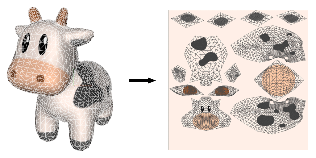
Texture mapping of a cow model
For this example there are multiple images being mapped onto the cow but the main idea is we are mapping the color of the image to the object.
Part 4: Barycentric coordinates
In this part of the project we are working on interpolating over triangle surfaces. We use barycentric coordinates to interpolates the color at a certain point. Barycentric coordinates, an important concept to this part, can be used for both interpolation and to see if the point is within a triangle.
Barycentric coordinates are used to show the position of a point relative to the triangle’s position using three scalars. To compute the position of this point using barycentric coordinates we use the following equation:
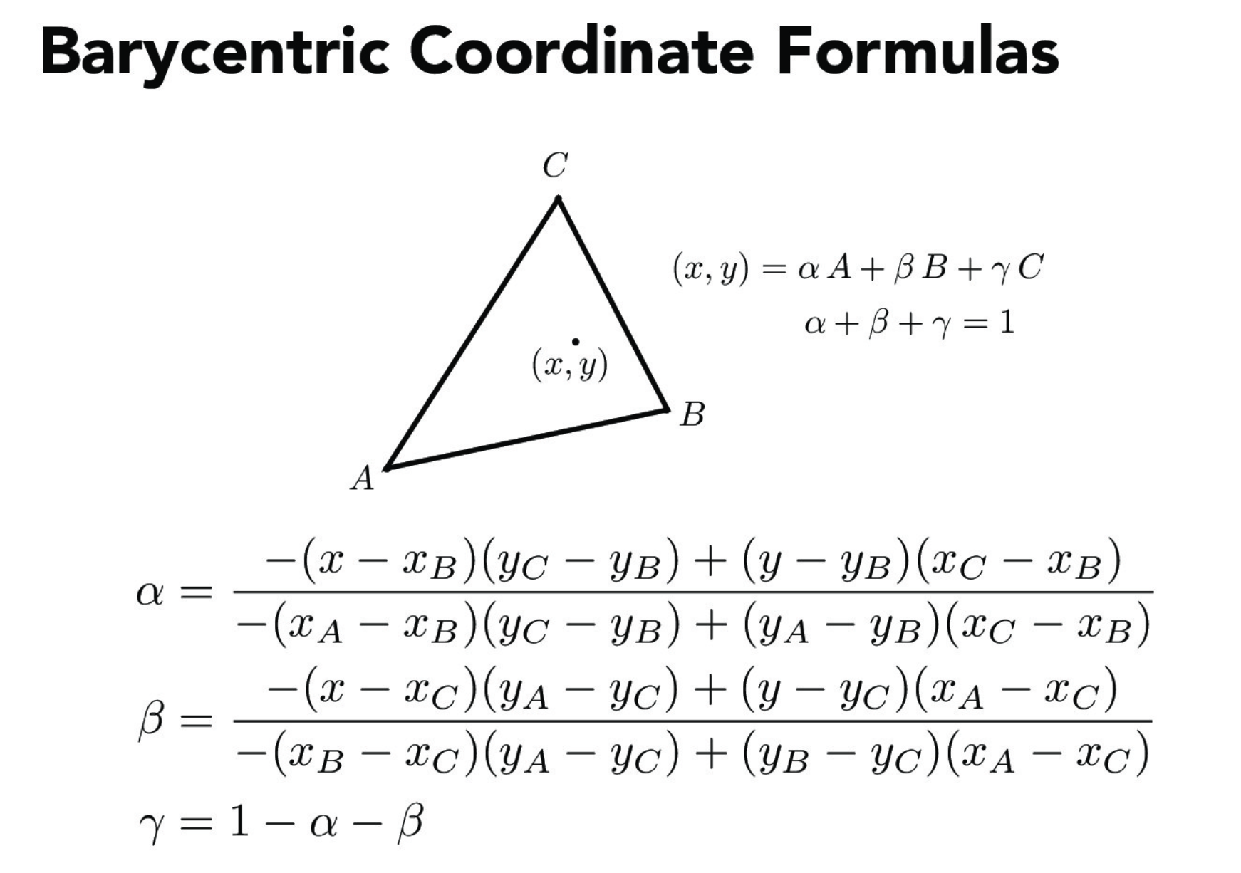
Barycentric equations
where A, B, and C are the vertices of a triangle and α, β, γ are the barycentric coordinates all of which sums up to 1 hence we can find γ by the last equation.
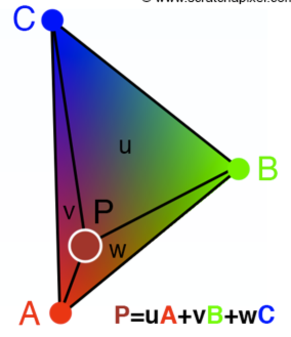
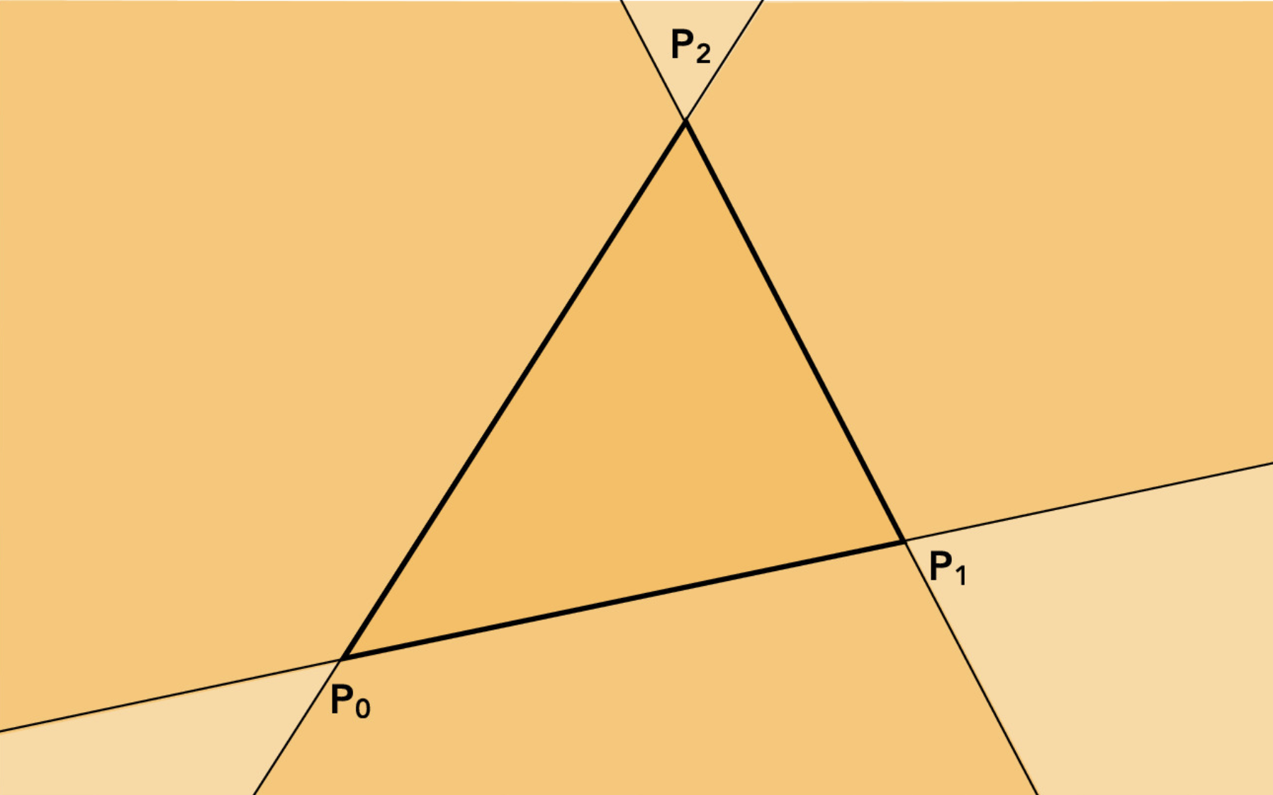
Barycentric coordinates on a triangle
In the example above we can think of the vertices each having a certain color: A being red, B being green, and C being red. The weights u, v, and w on the triangle are used to interpolate vertex data at point P. Because P is closer to A, u will have a higher value than v and w. So the color of point P is closer to red. as shown in the center circle.
The point (x, y) is within the triangle (A, B, C) if 0≤ α, β, γ ≤1. If any one of the coordinates is less than zero or greater than one, the point is outside the triangle. If any of them is zero, the point is on one of the lines joining the vertices of the triangle.
A simpler way to think of barycentric coordinates is to think of strings at the end of the vertices of the triangle. The “heaver” the weight is the closer the point is to that vertex.
Below is an example of an image I used barycentric coordinates for to demonstrate a smooth color gradient.
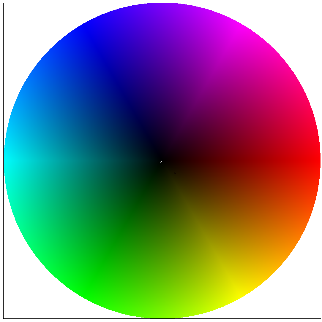
Texture mapping of a cow model
Part 5: "Pixel sampling" for texture mapping
The concept of texture mapping involves finding the corresponding pixel between the texel. The difficulty of this part is often times there is no one to one mapping from texel sampling rate to pixel sampling rate. This is due to minification, when there is one pixel sample per multiple texel samples, and magnification, when there is many pixel samples to one texel sample. In this section important concepts are bilinear filtering and nearest-pixel filtering. In this part of the project, we continue to use barycentric coordinates to calculate the sample texture value for texture mapping. To tackle the jaggies and moire pattern, we use texture antialiasing such as bilinear filtering and nearest-pixel filtering. Nearest-pixel filtering takes the texel closest to the pixel’s (u, v) coordinate and sets the texture of the pixel. Bilinear filtering takes the texture values of the 4 closest sample locations and uses linear interpolation to get the resulting value. So when taking the texture sample of a given pixel, we first get the (u,v) coordinates of the corresponding texture space. We then pass in these coordinates into sample, scale this point to mipmap’s width and height. Then, using this point we find the texel at this point. Finally, we return the interpolated color. (In bilinear sampling the only difference is we find the 4 neighboring points around the (u, v) coordinate and interpolate based on these points.
Below is the process of bilinear filtering. We take the linear interpolation of the horizontal pairs of neighbors (top 2, bottom 2). Then using the result of these 2 linear interpolations we find the final linear interpolation and get the result from this.
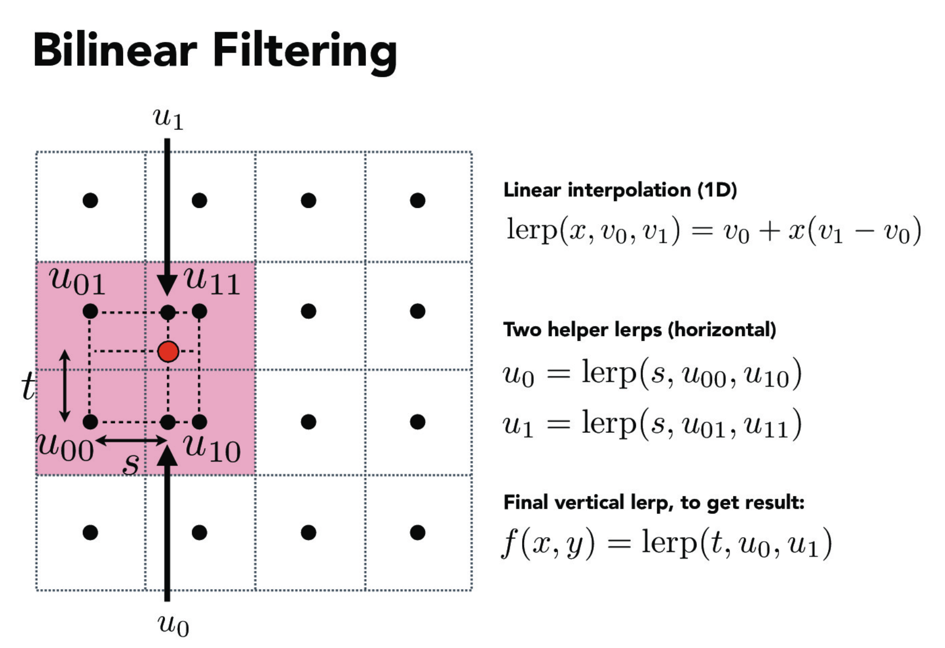
Bilinear filtering
Below are examples of the differences of bilinear filtering versus the nearest pixel sampling under different sample_rates.
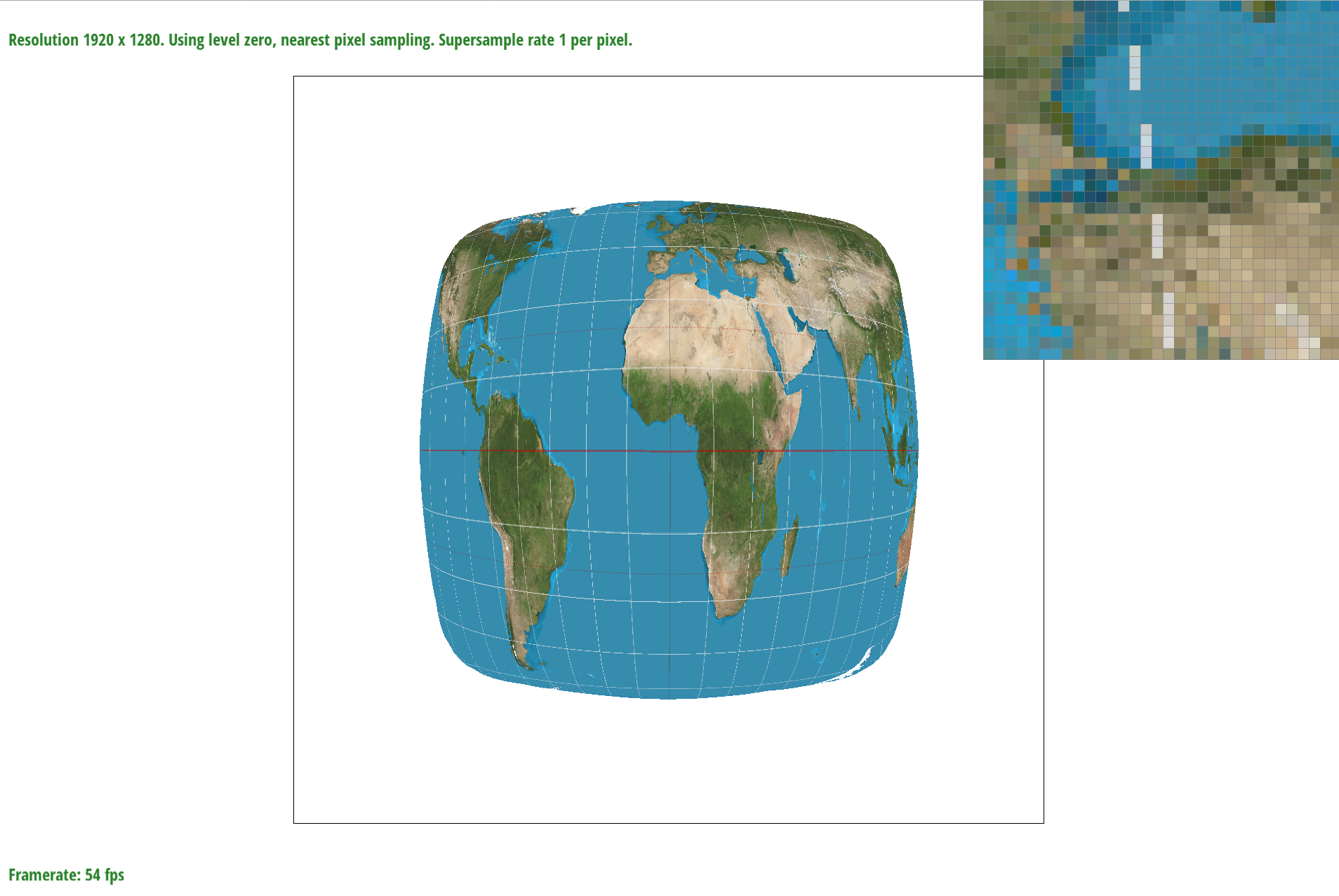
nearest sample_rate = 1
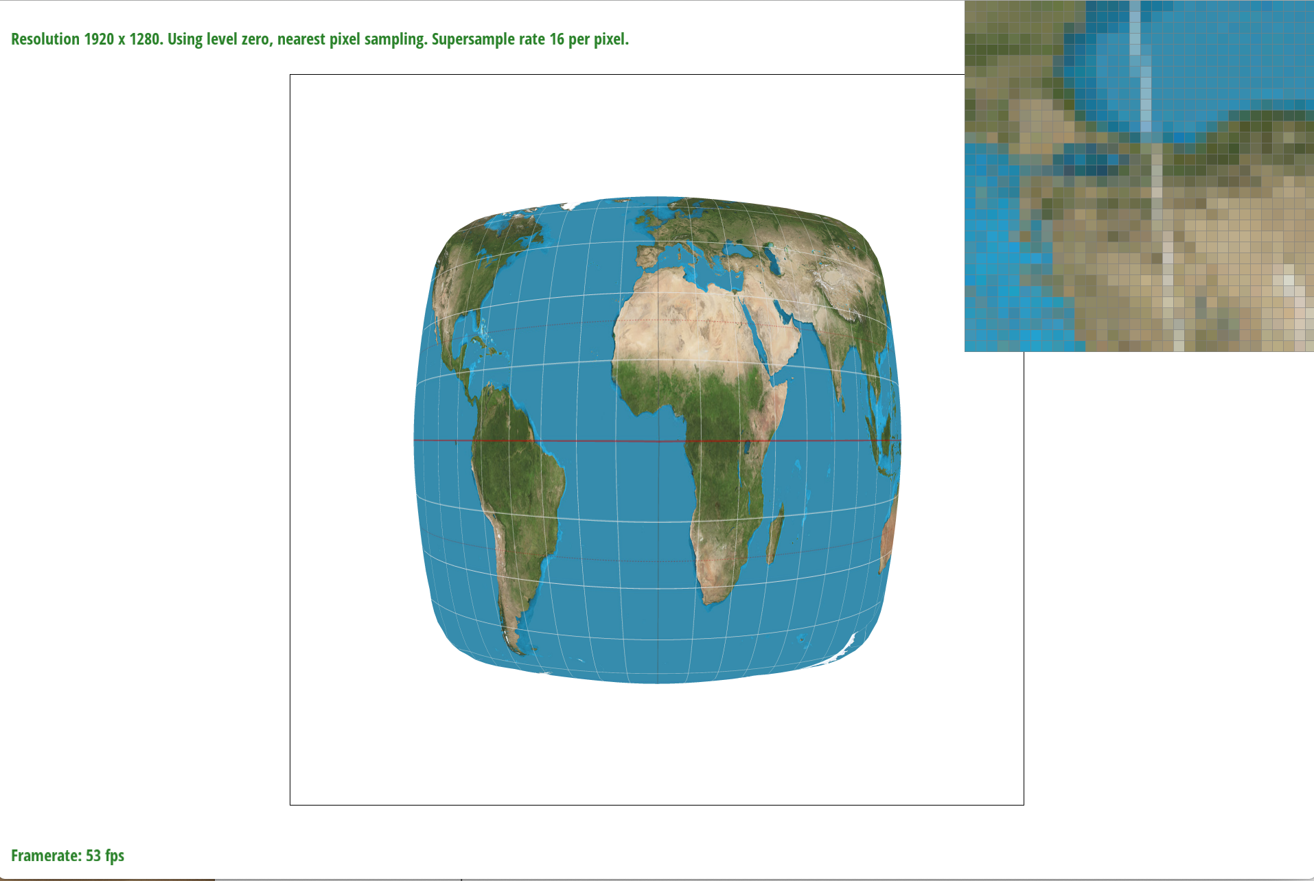
nearest sample_rate = 16
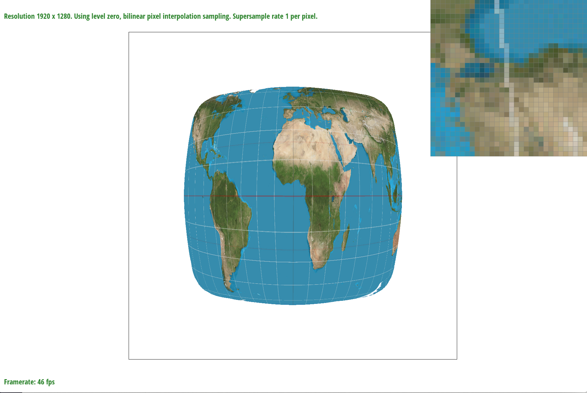
bilinear sample_rate = 1
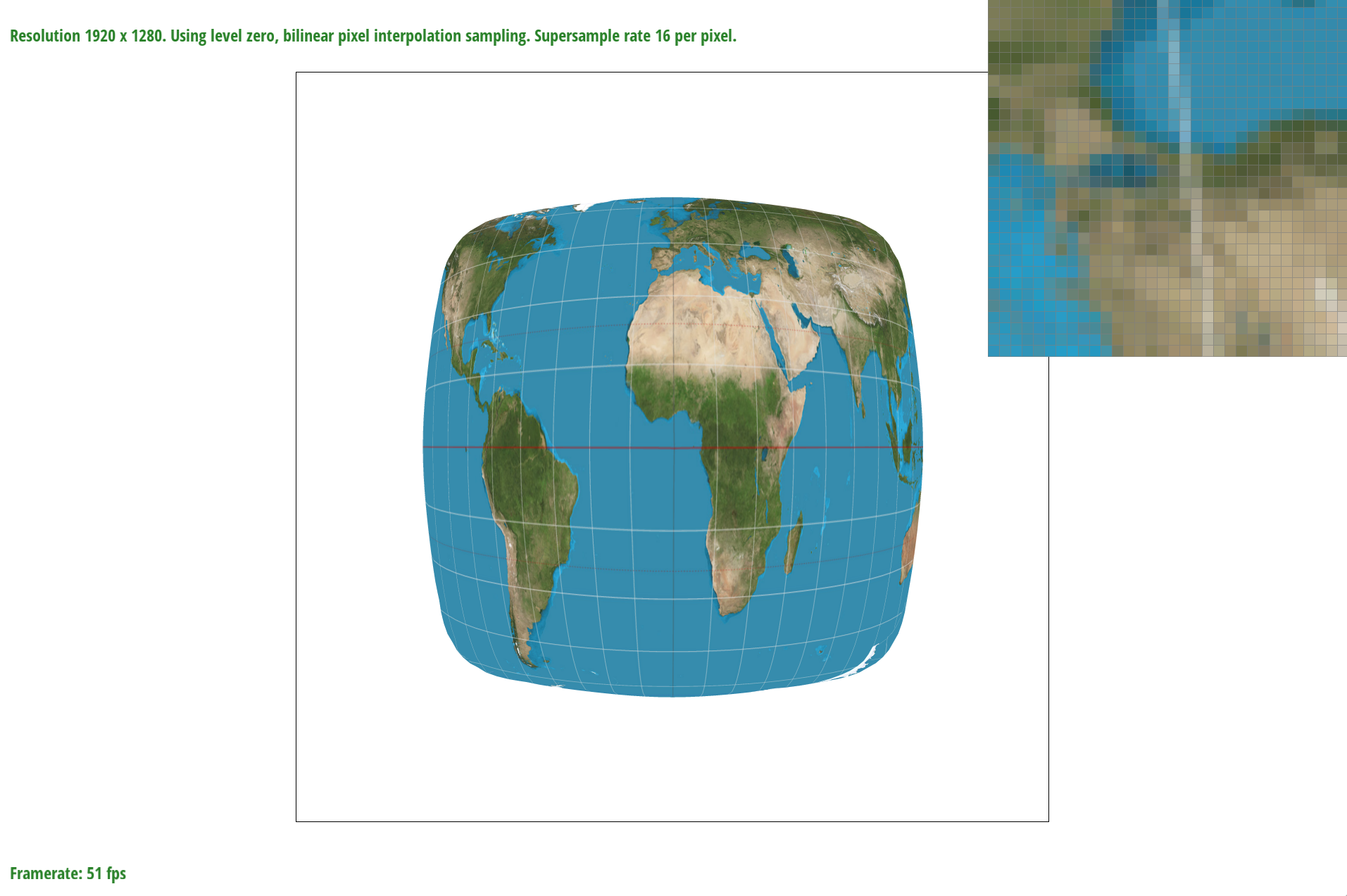
bilinear sample_rate = 16
In the examples above, you can see the differences between bilinear filter and nearest filtering. In the sample_rate = 1 example the nearest example has a separated longitudinal line while in the bilinear example the longitudinal line is connected. To demonstrate the difference of bilinear sampling at a higher sample_rate, both lines are connected however in the nearest example it looks like there are some texels that are missed. In the bilinear sampling it is however blurrier but is less of a “lost” texel look. When rendering these images there was an obvious delay when using bilinear filtering.
Part 6: "Level sampling" with mipmaps for texture mapping
In this part of the project we incorporate level sampling from mipmap levels as oppose to directly from the texture. The importance of this is to optimize computation and prevent distortions from happening. In this part of the project, I use the mipmaps hierarchy to better represent the texture mapping. At different levels of mipmap are different texture maps at different downsampled scales.
Implementing part 6 is very similar to part 5 with the exception of using levels. Like how we found barycentric coordinates to interpolate colors, I mapped a coordinate in the triangle to the uv texture coordinate. I calculate how far (x+1,y) and (x, y+1) end up being in the texture plane. To determine the level of texture to be mapped is based on the distance between the neighboring pixels under the (u,v) coordinate. If neighboring pixels are mapped to farther texture coordinates than the mesh doesn’t need to be high resolution. This means we use the downsampled version of the map. However, if it is close then we use the original texture map. Then, rather than having to generate the whole texture, the best mipmap level is passed for pixel interpolation
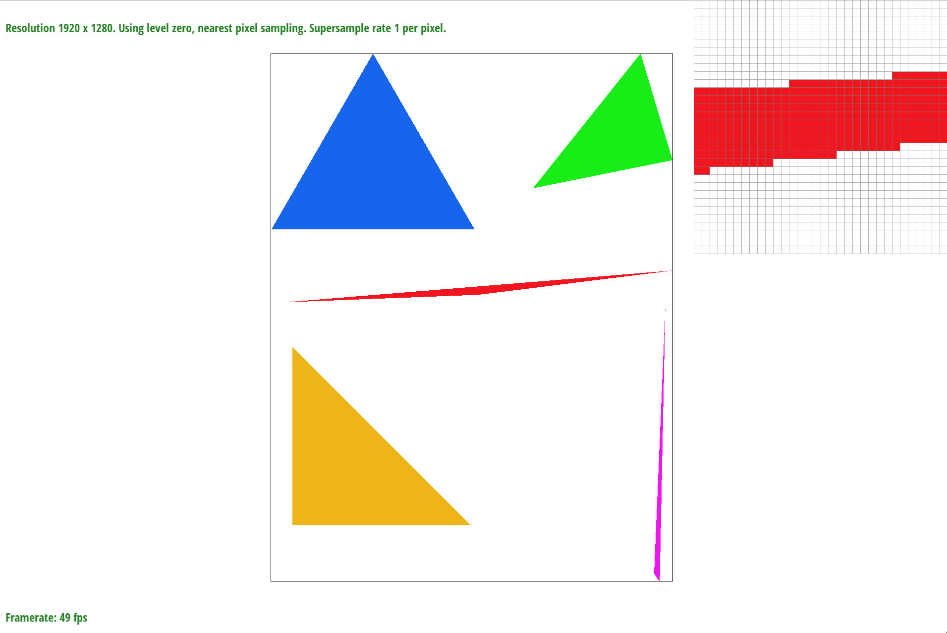
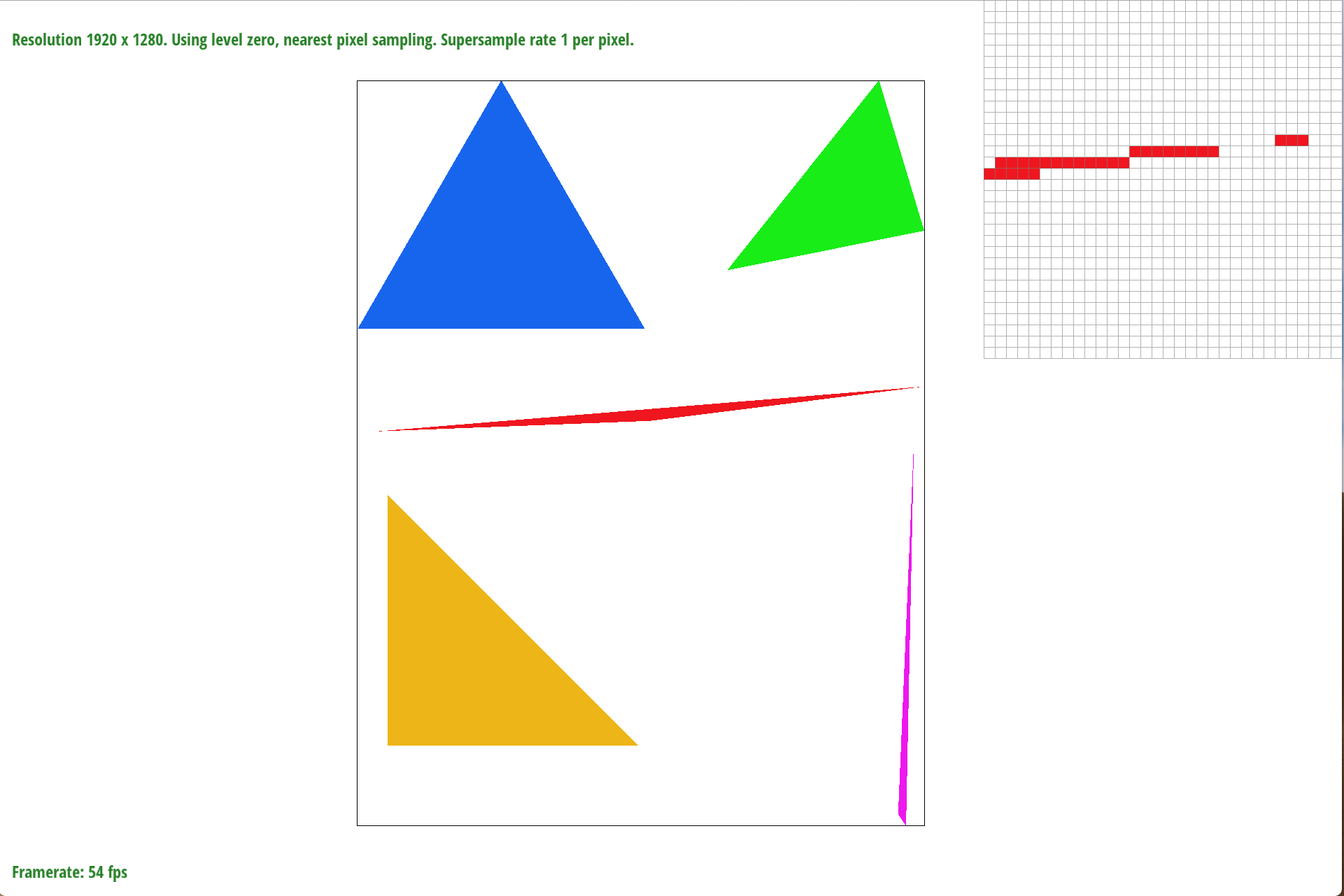
Below I generate the differences of the 4 combinations of level zero and nearest with one of nearest and bilinear sampling.
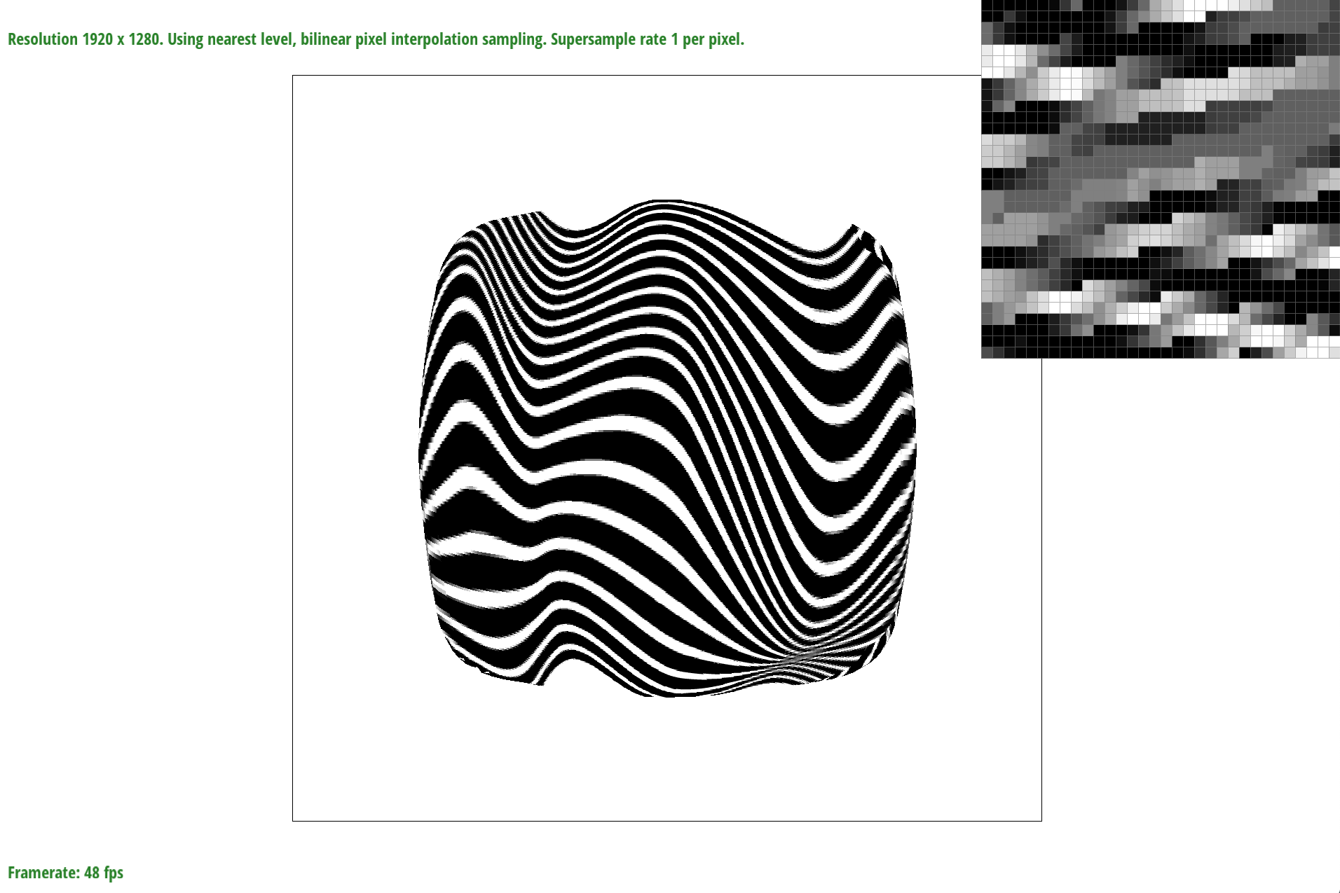
L_nearest P_linear

L_nearest P_nearest
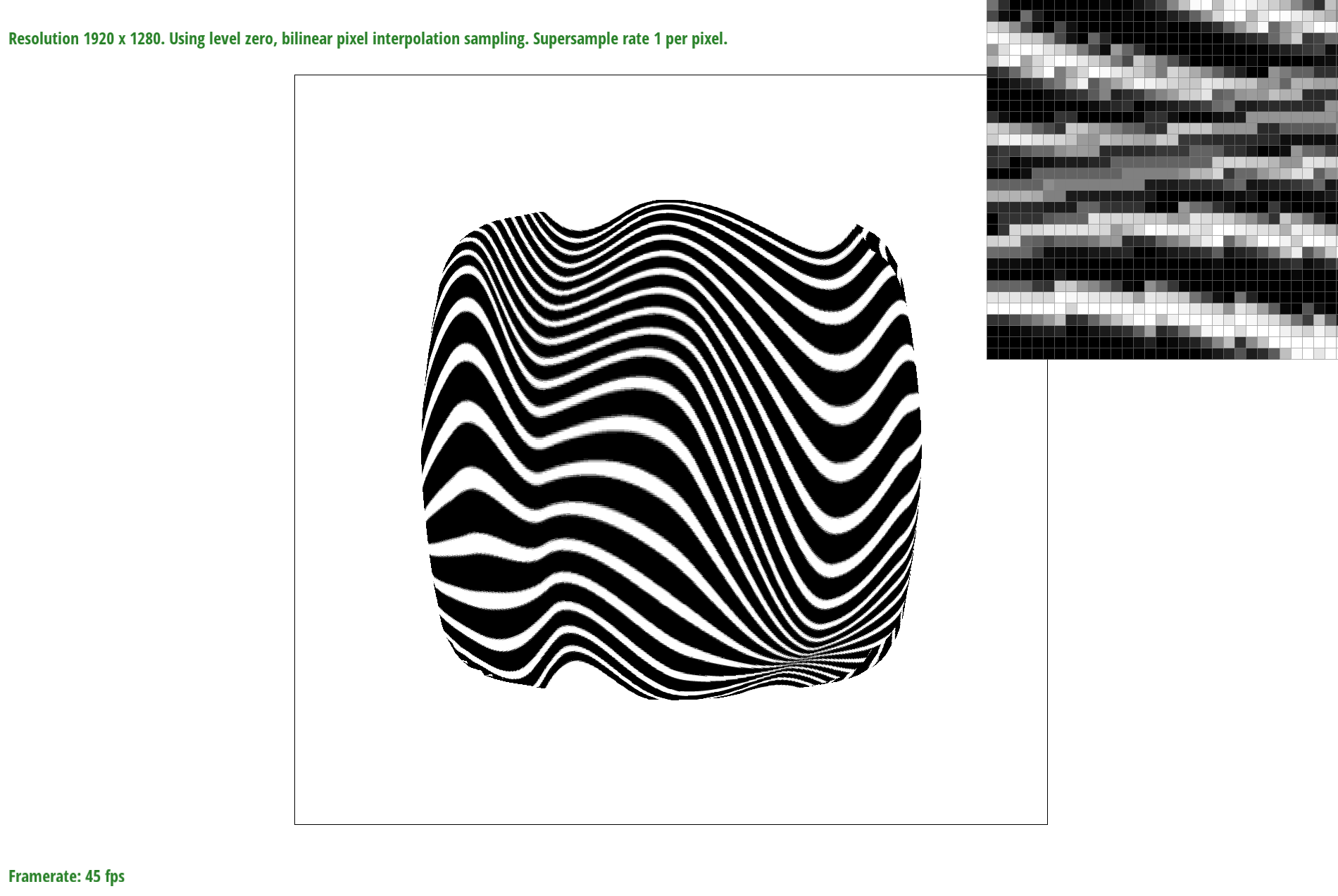
L_zero P_linear
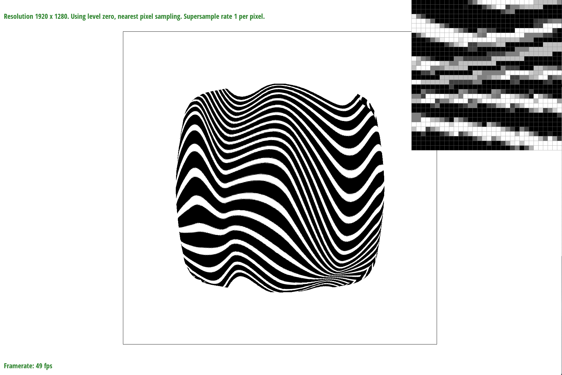
L_zero P_nearest
Using different antialiasing methods has its benefits but also downsides. When rendering the images, it didn’t take much longer than point sampling. Bilinear sampling’s antialiasing looked better. Level zero sampling takes the most memory because it doesn’t use mipmaps. Nearest isn’t the best option for antialiasing but is fast. Level sampling has to store extra leveling but is a great method for antialiasing. Bilinear sampling with level 0 looks the best zoomed out and level 0 with nearest looks the best zoomed in.