Abstract

Fluid simulation is used in many applications such as films, games, and research. In this project, we build a 3D position-based particle simulator. We closely follow NVIDIA’s paper published by Macklin and Muller. This paper provides a Position Based Dynamics framework which improves the Smoothed Particle Hydrodynamics framework. Implementing incompressibility, which is a term for constant fluid density, with SPH is expensive because it requires small time steps to simulate large forces, but the PBD framework allows for stable and faster performance for real-time fluid simulation.

In this paper, we review our technical approach and present our results in our final video.

Technical Approach

This project closely followed the Macklin and Muller Position Based Fluids paper. We first set up the environment we borrowed from the open source code from CMU. This set up 6 plane box with a GUI that allowed us to screenshot and start/stop the simulation. We then applied the gravitational force to simulate a basic particle drop then handled collision so that the particles stayed within the box. We then implemented based on 2 resources, from the Macklin and Muller paper and other extensions from outside resources.

From Macklin and Muller

Incompressibility

To improve particle distribution and surface tension, we first implement incompressibility by enforcing constant density on each particle. Between each particle and its neighbors was a function of the constraint. Below we define the equation of state:

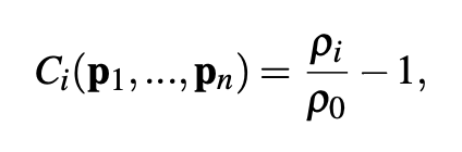
where ρ0 is the rest density and the ρ1 is the the SPH density estimator given by:

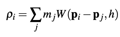
using the Poly6 kernel for density estimation and the Spiky kernel for the gradient calculation. We derive the gradient function with respect to a particle k:

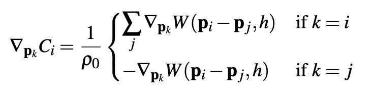
In the above equation, we cover 2 cases: whether k is a neighboring particle (k = i) or not (k = j).

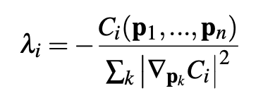
When we combine the density estimator and the gradient of the constraint function, we are able to calculate the lambda value:

Tensile Instability

Another issue we resolve is particle-clustering which happens when there is a negative pressure when there are too few neighboring particles unable to satisfy the rest density. We resolve this by adding an artificial pressure in terms of the smoothing kernel:

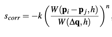
where ∆q is a point at some fixed distance inside the smoothing kernel radius and k is a small constant.

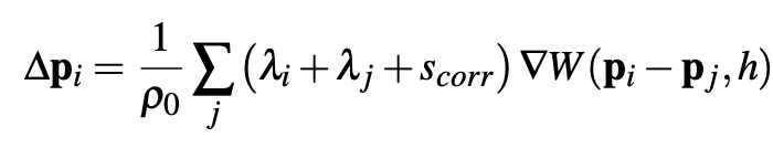
When we include this in the particle position update we get:

Vorticity Confinement

When using position based methods, an additional dampening on particle movement is added. We use vorticity confinement to replace this lost energy. This adds a spiral movement to the particles which makes the simulation look more realistic. We first calculate the vorticity at a particle’s location using:

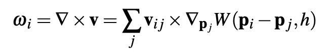
We then calculate a corrective force using the location vectors

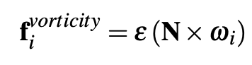
where N = η / |η| , η = ∇|ω|_i, and a low ε constant.

A challenge here was finding η, which is the gradient of the magnitude of a particle’s vorticity, because our particles form a discrete space with a non-uniform distribution. We tried importing AutoDiff libraries that use dual numbers for forward automatic differentiation, but ended up using a finite difference method.

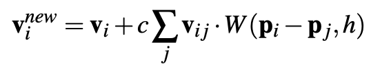
XSPH Viscosity

For coherent motion in our simulation we implement XSPH viscosity, which smoothes over differences between neighboring particles’ velocities:

Extensions

Spatial Acceleration Structures, K-D Trees

One important area of optimization is in neighbor-finding, which needs to be done each time step to make it easy to update particles based on a given neighbor range (defined by the kernel width constant for each kernel function).

We started with a simple 3D spatial hashmap, almost exactly like the one implemented in our class projects. The downside to hashmaps is that in vanilla scenes, gravity pushes particles down and thus pushes the particle distribution to be heavily skewed toward low y values. In this case, we’d like the hashmap to be able to dynamically size its cells based on observed particle distribution.

At first we tried to add a logarithmic scale to the y axis of the spatial hashmap, but this was not effective and not general. Following this, we decided to use K-D Trees instead.

The K-D Tree implementation we went sorts the particles and uses their true median as the splitting point. This led to worse runtime than spatial hashmaps, so we added a optimization found in research papers which randomly samples k particles, sorts them, and uses the median of the samples as an estimate of the true median.

Our optimized K-D Tree performed similarly to spatial hashmaps, but with much higher variance. When the particles are extremely spread out in space, the hashmap was 10-20 percent faster. When the particles are compressed and skewed in space, the hashmap was 5-10 percent slower. Runtime was found by measuring the time it took for each time step.

Macklin and Muller use CUDA for parallelized nearest-neighbor search, which would be a great addition to our project (none of our members had CUDA experience and there was already plenty to learn).

Custom Meshes

While the starter code included a mesh of the bunny at a few different resolutions, we also wanted to experiment with initializing blocks and sheets of fluid.

By building the mesh programmatically, we can fit it to the dimensions of our scene environment; more importantly, we can control the particle count and distribution

We also tried importing standard obj meshes from: https://people.sc.fsu.edu/~jburkardt/data/obj/obj.html, but none were a great fit (either had too many or too few particles).

Dynamic Scenes

We implemented moving walls to simulate a wave pool effect and get a better sense of how the particles act in highly dynamic environments. We also tried implementing a fountain our spout of fluid shooting into a scene, but the results were unsatisfactory.

Both of these dynamic scene types were drawn from classic fluid simulation scenes.

Collision Objects

We implemented fluid collision with planes and spheres to simulate interaction beyond particle-to-particle.

Problems Encountered

During implementation, we encountered a few technical problems.

Setting Up the Environment

At the milestone, we decided to take a pivot and change the environment of the project. Instead of building an environment from scratch we decided to switch over to open source code from CMU which helped us focus more on the algorithm. The open source code was meant for a Windows or Unix machine, and we all had MacBooks. We spent a lot of time on trying to get the code to build. We were able to debug necessary libraries in order to successfully build the project.

Sphere protruding through edges

Below demonstrates one of the issues we were running into during simulation. The particles closest to the edges were protruding through the edges. The solution to this problem was a quick fix with collision based on the center and radius of the particle in respect to the position of the edge.

Explosion

Below demonstrates one of the issues we were running into during simulation. When the water particles lose the bunny figure, it exploded upwards, producing unexpected behavior. This is likely due to constant values which have not been tuned perfectly to the scene. While we did try various combinations of rest density and different force constants, long simulation test time and high variation across scenes made this difficult to do manually. An automatic parameter tuning tool would have been useful here.

Takeaways

One of the key lessons we over the course of this project was how to navigate through and parse a technical academic research paper. Understanding complicated mathematical formulas and translating concepts into functioning code that models similar results proved to be an interesting and difficult challenge.

Another key learning was around setting up a functioning repository structure, navigating Git and CMake configurations, and working with three different people within a single project structure. In the course of the project we also learned a lot about fluid dynamics and particle interactions. Finally, we have a newfound appreciation for the power of the GPU and the incredible speedups possible due to parallelization that made real time graphics and rendering a reality.

Looking back at our approach to this project, we found there were hard decisions we had to make and things we could have done differently. Comparing our final results to our initial proposal, we noticed there was a significant change. At the beginning, we were very excited to implement a lot of features into our project. However, we ended up spending a lot of our time trying to just learning the material and realized we needed to focus more on the important algorithms first before implementing the nicer features. We underestimated how long it would take to fully understand and implement the algorithms. Looking back we could’ve improved on planning and sizing the project.

Initially we made the decision to build the project from scratch. However, we figured there was a big learning curve to WebGL let alone the algorithm. So midway through the project we made the pivot from creating the project from scratch to using open source code from CMU. This helped with shifting our focus from setting up the project to implementing the algorithm instead. This was a big change but I think it helped with making sure our time spent on the project was more productive.

There were several underlying concepts we learned from both the Macklin and Muller paper and other resources. There were many math and physics concepts we were unfamiliar with and needed to learn to have a foundational understanding of the project. Although we were implementing a project from a paper, there were other concepts that we were not explicitly written and needed additional information about. The Macklin and Muller paper gave a good high level understanding of the concepts but in-depth details needed more research.

Lastly, using technology we were unfamiliar with needed extra time to learn as well.

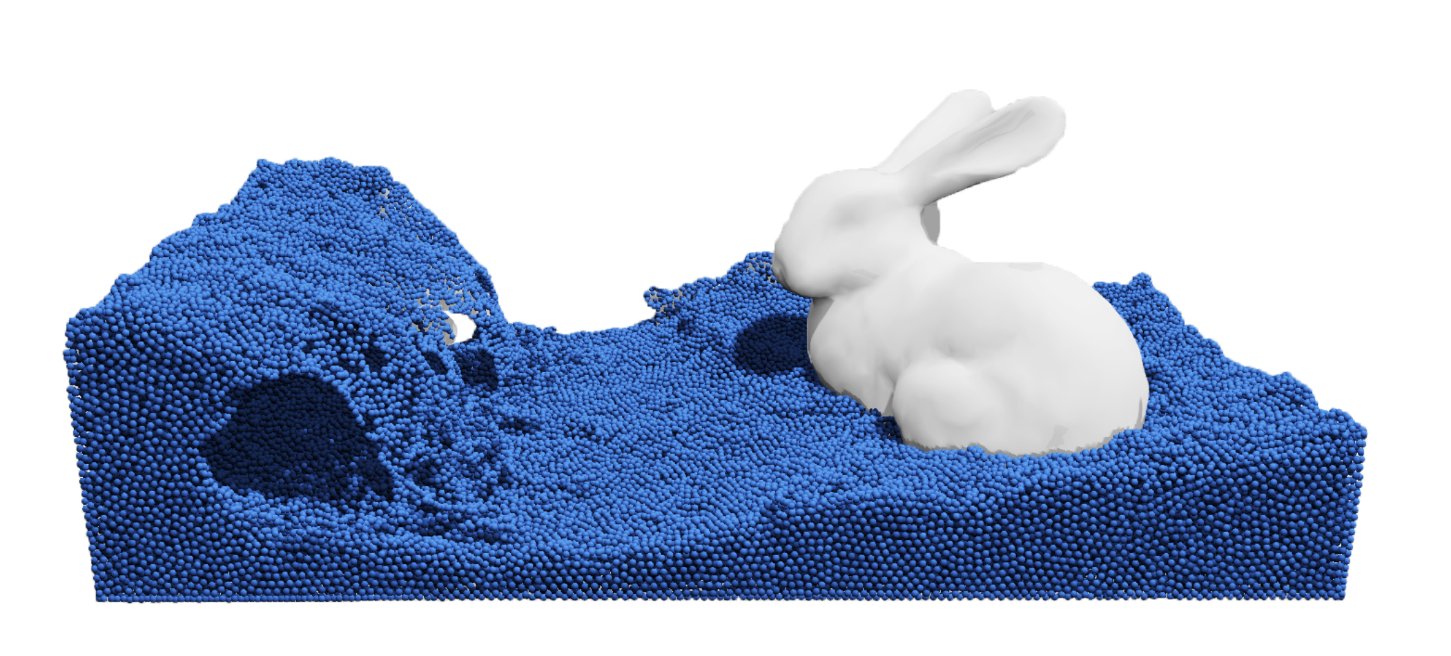
Results

Below are results from our simulation.

Initial Simulation

This is the initial simulation with gravitational force only and no collision handling.

Final Simulation

After implementing the algorithm from the paper and additional features, this is the final simulation.

Bunny XSPH Viscosity and Vorticity Confinement

Below is the comparison of without (Left) and with (Right) XSPH Viscosity and Vorticity Confinement. There is a very subtle difference -- in the left simulation the particles are less cohesive and exhibit more bouncing behavior. In addition, there is unnatural vibrating behavior of the particles on the left edge on the left box. After implementing XSPH Viscosity and Vorticity Confinement these weird behaviors are handled.

After perfecting the simulation we experimented with dynamic scenes.

Dynamic Scene Effects: Example 1

In this example, there is an upward gradient on the bottom part of the box. The left side of the box is moving pushing the particles creating a wave like simulation.

Dynamic Scene Effects: Example 2

In this scene the floor is divided into a ‘v’ shape. The mesh is initialized as a flat sheet of particles—note that the effect of the sheet spreading out before it contacts any surface is a visualization of the effect that rest density and the other constants have on the simulation.

Collision with Rigid Objects

Below is an example of fluid collision with a sphere.

References

Macklin and Muller: “Position Based Fluids” Paper
Assignment 2: Position Based Fluids (CMU)
Github Repo

Contributions

Ashley worked on the milestone and final project write-ups, slides, websites and videos.

Jennifer worked on writing the project proposal, setting up the simulation environment on Linux, debugging errors in the basic fluid simulation, and implementing collision with rigid objects.

Z worked on writing the project proposal, implementing the algorithm from the Macklin and Muller paper, creating dynamic scene effects, and experimenting with spatial acceleration structures using a K-D tree.