Project 3: Pathtracer 2
Ashley Nguyen | CS184-agh
Overview
In this project, I add more features such as materials, environment lighting, and camera simulation.
Part 1: Mirror and Glass
In this part of the project I implement mirror and glass models with both reflection and refraction. The reflection
Below are pictures of the same picture with different number of bounces. With different bounces we are able to see different effects.
At max_ray_depth = 0, we only have direct lighting. This is why we can not see the spheres or the ceiling.
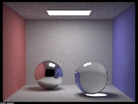
At max_ray_depth = 1, there is some reflection on the spheres. The mirror is mostly working like what we’d expect. The only thing missing on the mirror ball is the white reflection from the ceiling. The glass ball still looks a little dark. The only bounces we can see are from the bounces that are immediately reflected.
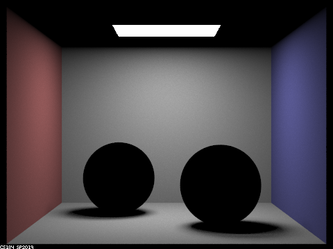
0 max_ray_depth
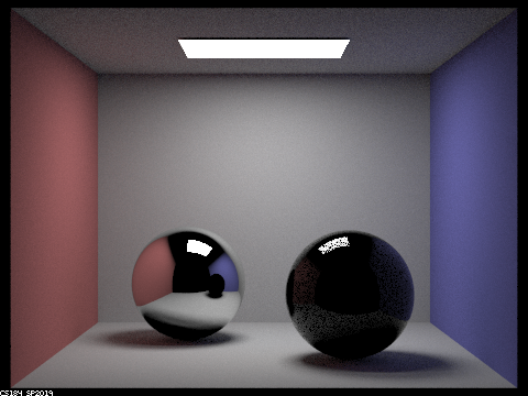
1 max_ray_depth
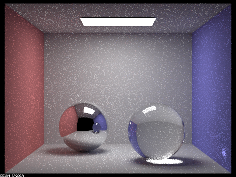
At max_ray_depth = 2, the mirror sphere we are now able to see the white ceiling being reflected. We also see the bottom the sphere is almost black and doesn’t look exactly like it’s supposed to. In the glass sphere, we are able to see through the sphere. However, it looks like the light is not able to go through the sphere.
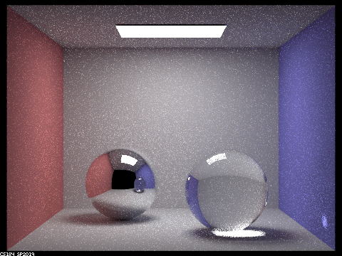
At max_ray_depth = 3, for the mirror sphere we see the reflection on the bottom of the sphere is lighter. The glass sphere now allows the light to go through and now illuminates the shadow. This action now shows because 4 bounces is needed from the camera to the floor then into the sphere then out the sphere onto the wall.
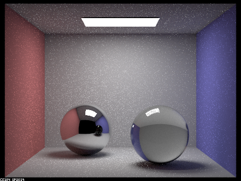
2 max_ray_depth
3 max_ray_depth
At max_ray_depth = 4, the mirror ball has not changed much except has gotten brighter at the bottom. With more bounces between the ball and the floor, this is how this is possible. The glass ball has now caused a bright dot on the blue wall.
At max_ray_depth = 5, there is not much change however there does look like there is more noise. This is the result of increasing the number of bounces. Because of this we get a more refractions and reflections causing this weird effect.
4 max_ray_depth
5 max_ray_depth
At max_ray_depth = 100, we see the details of the spheres looking closer to natural.
Part 2: Microfacet Materials
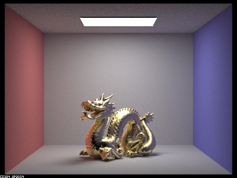
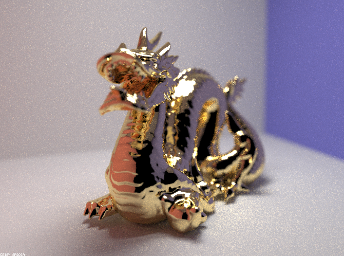
Below are examples of the dragon photo with various alpha values. The higher the alpha the more brushed the sculpture looked while the lower the alpha the more reflective and shiny the material looked. In addition, noise increased as alpha got smaller.
At alpha = 0.5, it looks very diffused and looks more brushed.
At alpha = 0.25, this is starting to look a little more shinier. It looks a little less brushed than the 0.5 picture.
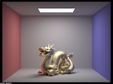
alpha = 0.5
alpha = 0.25
At alpha = 0.05, this has a lot more shinier material than the 0.25 example. In this pic, we also get a little more noise.
At alpha = 0.005, I get a lot more noise. The model has a mirror type of look to it; it is a lot more shinier and glossier.
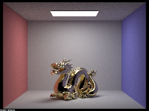
alpha = 0.05
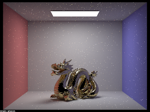
alpha = 0.005
Below is are rendered pictures of the bunny using uniform cosine hemisphere sampling and importance sampling. Using uniform cosine hemisphere sampling we get extra noise whereas in the importance sampling we have less noise and can see the material more clearly
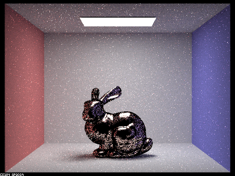
uniform cosine hemisphere sampling
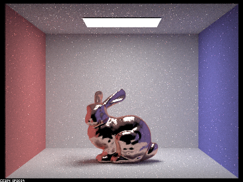
importance sampling
Below I rendered the same dragon image but using variables of an aluminum material. For eta I use [1.3352 1.0109 0.68955], for k I use [7.3398 6.6157 5.6471] and alpha I use 0.005.
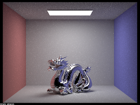
Aluminum
Part 3: Environment Light
In this part of the project I will implement an importance sampling scheme for environment lights. Environment lights with large variation in incoming light intensities will have significantly less noise with good importance sampling. The basic idea is that each pixel in the environment map gets assigned a probability based on the total flux passing through the solid angle it represents.
We used 2 different samplings: uniform and importance. Uniform sampling sampled a random direction on the sphere and checked the environment map’s radiance. Importance sampling was biased based on the concentration in the direction of bright lights. This significantly lowered the noise of the renders.
Below is the image of the environment we use. The image on the right is the probability_debug.png file which is generated using the function that initializes the probability distributions.
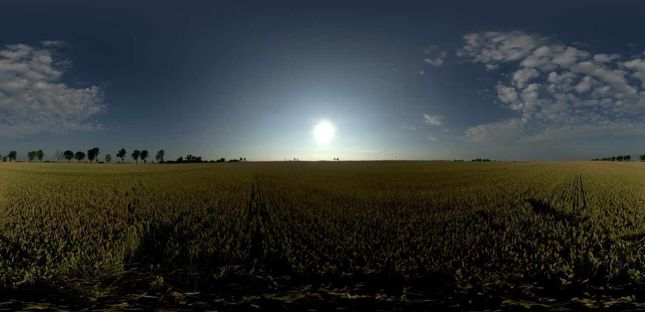
Environment File
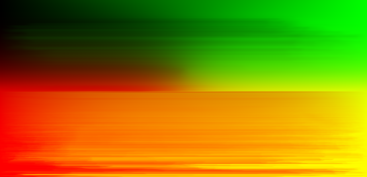
probability_debug.png
Below are the rendered images of bunny_unlit.dae. The uniform sampling image is a little more noisier than the importance sampling.
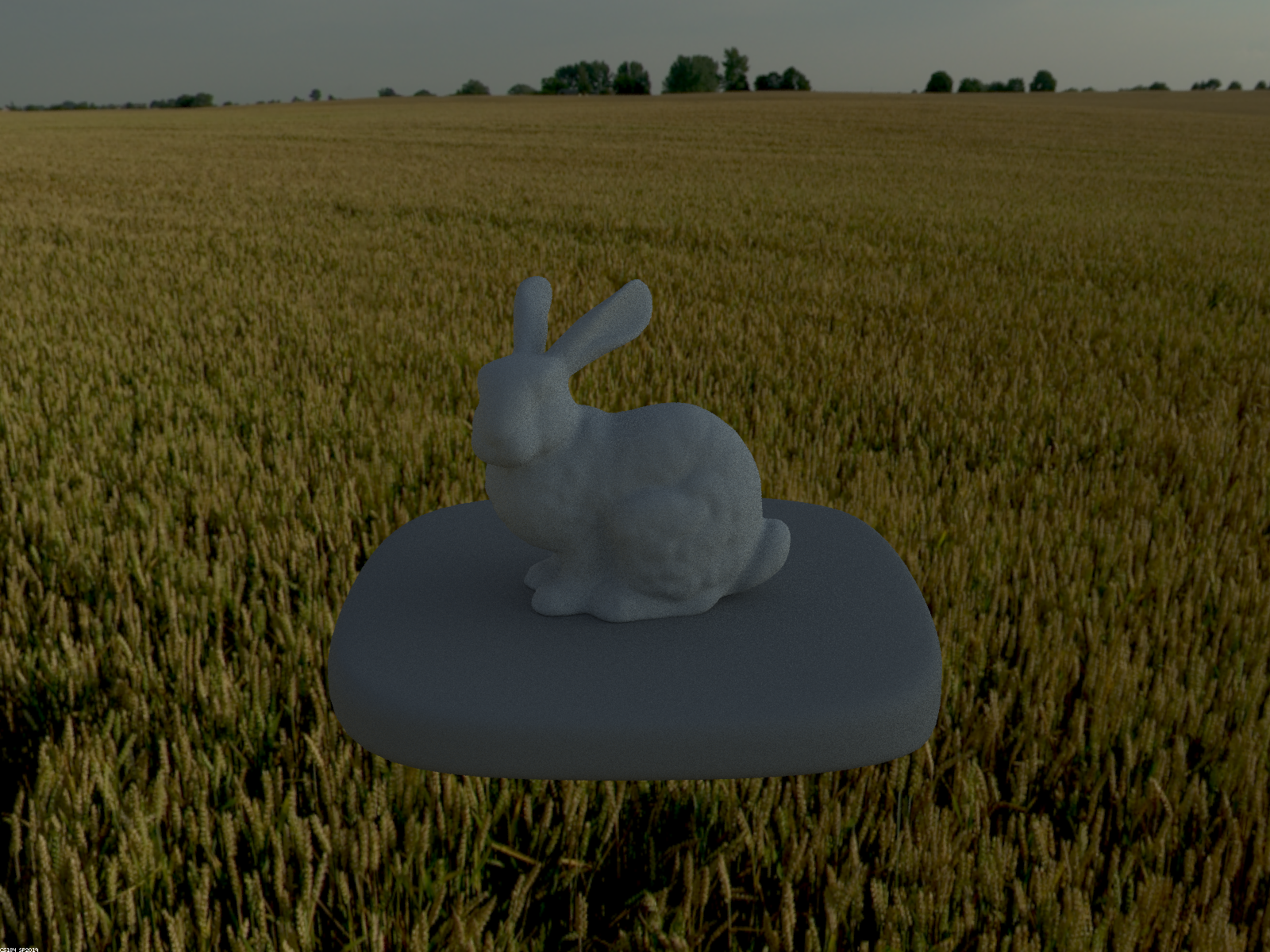
Uniform sampling
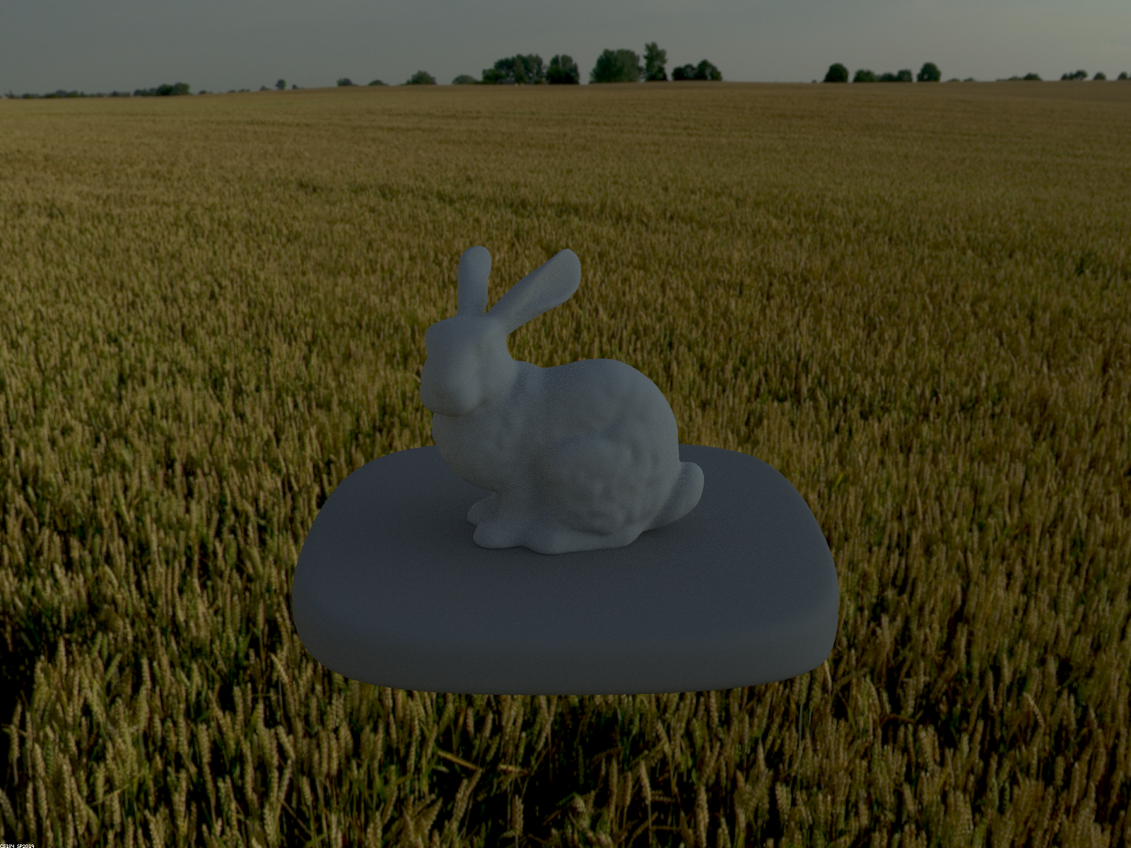
Importance sampling
Below are the rendered images of bunny_microfacet_cu_unlit.dae. The uniform sampling image is a little more noisier than the importance sampling. In addition, the importance sampling looks a little more shiner and the details of the model look more detailed.

Uniform sampling
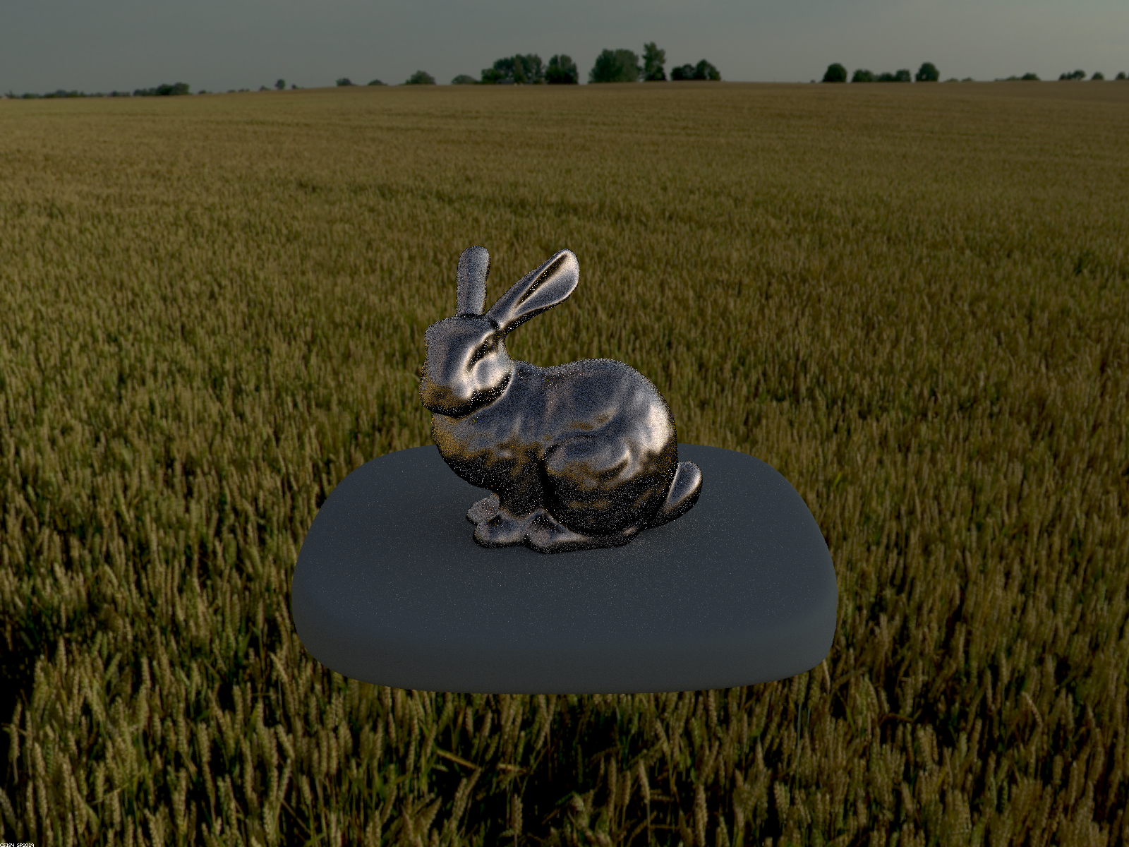
Importance sampling
Part 4: Depth of Field
The pinhole camera model everything in the camera is in focus. On the other hand, a thin-lens camera model simulates the effects a real camera will create. A camera normally focuses on one point of the image and refracts on other points.
Focus Length
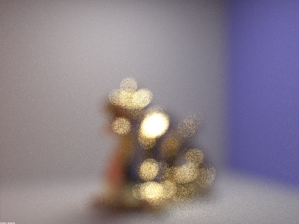
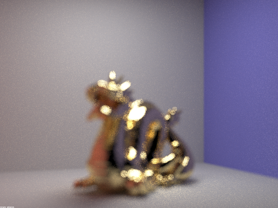
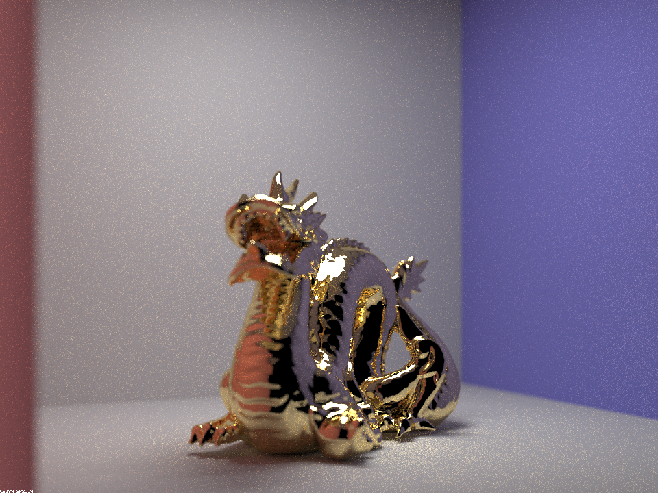
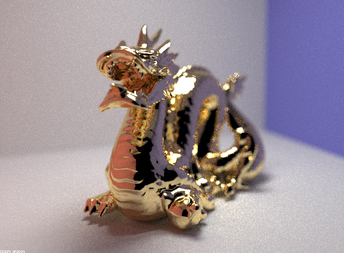
Below are images of various focal length. This focuses on different parts of the model.
focus length = 0.5
focus length = 1.2
focus length = 3.2
focus length = 7.2
Aperture Sizes
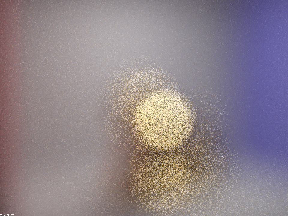
Below are images of various aperture size with the same focal length. The image gets blurrier and the depth of field becomes shallower.
aperture = 1.2
aperture = 1.25

aperture = 1.3

aperture = 1.35